Traveling Salesman Problem (TSP)
Contents
- 1 Introduction
- 2 Software Installation and Data Downloads
- 3 The Tutorial
- 3.1 Getting Started: GRASS Database (just minutes)
- 3.2 Importing .shp
- 3.3 Importing .csv
- 3.4 Processing in Grass
- 3.5 Network Preparation
- 3.6 Extract a Start point
- 3.7 Attribute Editing
- 3.8 Connect Customers to the Network
- 3.9 Network Analysis Examples: Shortest path, no cost
- 3.10 Network Analysis Examples: Shortest path, with costs
- 3.11 Network Analysis Examples: Traveling Salesman Problem
- 3.12 Network Analysis Examples: Want more? Here is another great tutorial
- 4 View results in Google Earth
- 5 Data
- 6 Conclusion
Introduction

This is a Free and Open Source Software for Geospatial (FOSS4G) inspired tutorial. It focuses on Network Analysis using a Geographic Resources Analysis Support System (GRASS).
About the Tutorial
This tutorials' main aim is to be clear and understandable. I made every effort to use real data even though this presents many problems. However, it is a reality that data is dirty and software is fallible. This tutorial will be very time consuming to complete, however, you will learn a lot along the way and this knowledge will easily transfer to future projects.
In this tutorial you will
- Install GRASS
- Download and prepare data
- Start a GRASS database
- Build a network and perform analysis on it
Note If the command line is not working and you don’t wish to take the time to troubleshoot this problem I have been given a great work around from my teacher Scott Mitchell. If you do not have GRASS folders set up refer to step named Getting on our way.
- 1. Launch the OSGeo4W
- 2. Type grass64 –gui and then hit enter on the keyboard. (notice there is a space between 64 and the dash)
- 3. You will see the old GRASS version load, so simply click File from the menu bar and click Quit GIS Manager.
- 4. Now in the command box type g.gui gui=wxpython&
Software Installation and Data Downloads
Software Installation

Install OSGEO Package (30-60mins)
First, you will need to install free geospatial software. I am mainly using GRASS 8.4.0 (originally created using 6.4.2). This can be found through the secure and trusted site of Open Source Geospatial Foundation OSGeo4w is Your Open Source Compass for Windows This package provides a set of open source geospatial software for a Win32 environment. Simply follow the directions from this site: Click Here to go to Download Page The great thing about this pkg is that is contains several versions of GRASS. So if something doesn't work in one version it might work in another.
Grass Tutorials
Grass Tutorials This website has tutorials on Getting Started and a variety of other tutorials with different difficulty levels. The getting started tutorials allow for an increased understanding of the software, though it is not necessary to complete it in full.
Data Download
To get started we need to download data required for the tutorial.
- Go to The City of Ottawa, Open Data Site
- Download the Wards 2022-2026 shapefile. You can find it here
- Download the Road Centrelines shapefile. You can find it here
- Download the Municipal Addresses csv file. You can find it here
Once downloaded, Unzip if necessary and add the unzipped folder to a folder named data and save it in a location that you will also ideally use to save the project.
- Make sure to rename all files in the wards layer to just wards.xx
- Also rename the municipal_address_point.csv to Addresses.csv
The Tutorial
Getting Started: GRASS Database (just minutes)

1. Open GRASS
2. Once opened. On the left hand side in the Data tab click on ![]() to create a new project.
to create a new project.
3. Within the "Define new GRASS project" tab, name the project and choose a location on your computer where you would like to save it. Click Next.
4. On the select Coordinate Reference System (CRS) page, choose "Read CRS from a georeferenced data file" and click Next.
5. You should now see a prompt asking for a georeferenced data file. Locate the folder in which you saved the data you downloaded from OpenOttawa and choose the wards.shp file.
6. Click Next and then Finish.
Now we are ready to start working in GRASS.
Next:Import data files and prepare them for processing and analysis
Importing .shp

1. You now have three screens open and running under GRASS. A command line black box, a GRASS GIS Layer Manager, and a Map Display pane. In the Layer Manager window click File | Import Vector Data |Common Import Formats.
1. You now have GRASS running with the GIS view and command prompt open in another window. In the GIS view along the top ribbon click File | Import Vector Data |Simplified vector import with reprojection [v.import].
2. A GUI window will appear to lead you forward. In the source input section browse to the data folder and choose Road_Centrelines.shp file and then run. If you watch the Layer Manager window it will tell you when all is complete. At the bottom of the window you will have to hit the Map Layers tab as you have been watching the command console tab.
3. Now the Roadways.shp file is loaded to the Layer Manager window simply toggle it on to view it in the Map Display window.
Next do the same for the wards.shp file.
Importing .csv
- This is not as straight forward as the .shp files. You must first open the Addresses.csv file in Microsoft Excel for editing.
- When Excel asks if you would like to remove leading zeros choose convert.
- Delete all columns in the table except for X, Y, OBJECTID, ADDRNUM, ROAD_NAME, and WARD
- The x,y columns need to be formatted. You can use the 'Find and Replace' tool. First replace all commas with periods. Then right justify the x and y columns. These are necessary steps.
- Save the file as a .csv. Excel might say that there is a problem, just ignore it.

- To bring it into GRASS:
- Click File|Import vector data|ASCII points/GRASS ASCII vector import [v.in.ascii]
- Under the Required Tab:
- Browse to the file and choose it. Then back in the GUI, name the output file.
- Under the Input Format Tab:
- Change the Field Separator to a comma ','
- Under the Points Tab:
- Number of header lines to skip: 1
- Number of column used for x: 5 (Make sure this number matches the column number in which your x values are located in)
- Number of column used for y : 6 (Make sure this number matches the column number in which your y values are located in)
- Number column used for category / id : 1 (Make sure this matches the column number where the global id is)
- Hit Run
Processing in Grass
- Type this in the command line box, it will adjust the region parameters.
g.region -p vect=Road_Centrelines
- Next extract the location you specifically wish to focus on. In this case it will be the Somerset ward.
v.extract input=Wards output=Somerset type=area where=cat=1
make sure that cat = 1 is the Somerset ward. You can check by opening up the attribute table of the wards layer and checking the cat value for Somerset ward.

- Next extract the customers that are within that ward from the larger customer data set.
v.select ainput=Addresses atype=point binput=Somerset btype=area output=addSomerset
operator=within
- Next extract the Road Centrelines
v.overlay ainput=Road_Centrelines atype=line binput=Somerset output=SomerRoads operator=and
Network Preparation
- Type this in the command line box, it will adjust the region parameters.
g.region -p vect=Somerset
- Next clean the data
v.clean input=SomerRoads output=SomerRoadCl type=line tool=break,rmdupl
Extract a Start point
- When you right click on the addSomerset layer in the Layer Manager window, select to view the Attribute table. Scroll to find the exact address you want to use and note its 'category' number, which will be the one in the first column for the row you choose, you will need to input that number later in the GUI. We will use the GUI for the next 2 extractions. Note: the category number may be the int_1 number
- :On the menu bar (Top ribbon) choose the following: Vector|Feature selection|Query with attributes
- :Once the tool is open browse to the addSomerset file and choose it for the input vector map
- :Name the output map as: Start
In the next tab: Selection (in the same tool)
- :In the types to be extracted section choose: point
- :In the Where conditions of SQL type section write the following: cat= category number (The point you chose in the first step)
If the above step didn't work change the cat= # to int_1= #. Or to whatever the field name is for the first field in your addSomerset layer.
- :click Run but do not close the window!!!
Next extract all other points minus the one we just extracted.
- :All you need to do is simply toggle back to the first tab to change the output name to Customers.
- :And then in the Selection tab: toggle on the Reverse Selection option and it will do the rest.
- :Hit run and close when done.
Attribute Editing
We know that the homes are not located directly on top of the roads so we must calculate and attach them to the network for processing and analysis. First we will create 3 new columns in the attribute tables and then populate them.
v.db.addcolumn map=Customers columns="x double precision,y double precision,dist int"
v.db.addcolumn map=Start columns="x double precision,y double precision,dist int"
v.to.db map=Start type=point option=coor columns=x,y
v.to.db map=Customers type=point option=coor columns=x,y
v.distance from=Start to=SomerRoadCl to_type=line upload=dist column=dist
v.distance from=Customers to=SomerRoadCl to_type=line upload=dist column=dist
Connect Customers to the Network
- Once we have the distance from all points to the roads,connect all the addresses to the road-network according to a threshold (distance)
v.net input=SomerRoadCl points=Start output=network_v2 operation=connect thresh=10
v.net input=network_v2 points=Customers output=net operation=connect thresh=50


- We can view information about the network
v.category net op=report
Network Analysis Examples: Shortest path, no cost
We have a start point, now it is time to choose a destination. Once again choose the 'cat#' of an address point, as you did earlier, using the attribute table from Customers.
v.extract input=Customers output=End type=point where=cat=44017
Open the Attribute tables for both the Start point layer and the End point layer.
Open Notepad to make a .txt file of these layer's x,y coordinates.
- Format is:

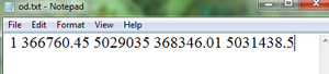

You will get the Start and End layer's x and y coordinates from their respective attribute tables. This is a finicky process, be sure not to put any extra spaces. Also do not hit the return key after you type the last number. If you do simply you the backspace key and delete everything up til the last number entered. Save the file as od.txt

v.net.path input=net output=route_nocost type=line file=od.txt
If you get an error then use the GUI found under Vector|Network Analysis|Shortest path. Or retype the code and in front of od.txt put its full address, like: file=/home/desktop/od.txt
Network Analysis Examples: Shortest path, with costs
First add two new columns to the network file.
v.db.addcol map=net columns='saftey int,cost int'
Next create at .txt file in Notepad
UPDATE Routes SET saftey=1 WHERE RD_SUFFIX='ST';
UPDATE Routes SET saftey=1 WHERE RD_SUFFIX='AVE';
UPDATE Routes SET saftey=1 WHERE RD_SUFFIX='CRT';
UPDATE Routes SET saftey=1 WHERE RD_SUFFIX='DRWY';
UPDATE Routes SET saftey=1 WHERE RD_SUFFIX='LANE';
UPDATE Routes SET saftey=100 WHERE RD_SUFFIX='PKWY';
UPDATE Routes SET saftey=1 WHERE RD_SUFFIX='PL';
UPDATE Routes SET saftey=1 WHERE RD_SUFFIX='PRIV';
UPDATE Routes SET saftey=100 WHERE RD_NAME LIKE 'HWY';
UPDATE Routes SET saftey=100 WHERE RD_NAME LIKE 'HIGHWAY';
UPDATE Routes SET saftey=100 WHERE RD_NAME = 'TURN LANE';
UPDATE Routes SET saftey=100 WHERE RD_NAME LIKE 'DRIVEWAY';
Now you can
- 1 Save the .txt as saftey.txt and then rename the extension saftey.sql and then use the command line to execute it, if you know the address.
db.execute input=/home/desktop/saftey.sql
- 2. OR you can open the GUI under the menu Database|Query|SQL statement
- Simply copy and paste the UPDATE arguments from above in the space provided, and hit run
- This is what I did but I had to do all steps in GRASS6.5 as it didnt work in 6.4.2
Now that the saftey column has been updated we can perform a cost related analysis. You will notice the non-residential like streets have a high cost and the residential have a low cost. The calculation will search for the shortest path with the highest saftey rating.
Now you can calculate with costs by either:
v.net.path input=net output=route_to_libraries_withcost file=/home/desktop/od.txt afcolumn=saftey dmax=10000
if you know the address of the od.txt file :

- OR by using the GUI at Vector|Network Analysis|Shortest path
Network Analysis Examples: Traveling Salesman Problem
If you have a set of points that you must travel to, extract them into a file of their own. Clean a new roads file for use in this section of the tutorial Connect the two layers (Network and set of points that you would like to travel to) as we did earlier
- Run a report on the network to discover the min and max of the second layer
v.category network name op=report
Run the Traveling Salesman Analysis
- put the min and the max from the report for layer 2. ccats=8-21 is just an example of how you should type it
v.net.salesman input=network output=salesman_nocost ccats=8-21
Network Analysis Examples: Want more? Here is another great tutorial
http://jcastellssala.wordpress.com/2012/05/07/basic-network-analysis-with-grass/
View results in Google Earth
You can export the various routes you have created in GRASS GIS and view them in free viewers like ArcView and Google Earth.
Export Vector Network Analysis Results to .KML
v.out.ogr input=Safest@PERMANENT type=line dsn=Users/MyName/Desktop/Safest.kml format=KML
- notice the dsn=Users/MyName/Desktop/Safest.kml It is very important to get this part correct. This is not a working address. I changed only the MyName part, everything else is correct to my computer. You will need to discover the address to where you wish to store your new file.
Data
- Go to The city of Ottawa, Open Data Site
- Download the .csv file Address Points (main) Or click this link. Note: When you unzip this file change its name to customers.csv.
- While at the same site download the Roadways.shp file and the wards2010.shp file too.
Conclusion
- Downloading and using the OSGEO4W package was very helpful. The following tutorial will teach you how to make more specific geospatial analysis. I fully believe that the skills you developed here will allow you to better navigate through other tutorials. Most problems I ran into had nothing to do with GRASS its self but more my lack of knowledge and understanding and the actual machine configurations that I was using. Knowing how to find the address of stuff on your own computer is important. Having python correctly linked to GRASS is very important to.
Contributions to This Tutorial
- Lluís Vicens taught me through his tutorial how to perform these calculations and answered my questions via email from Spain in less than 24 hours. He teaches his students that this is how things work in the world of FOSS4G. You can get results and you can be heard.
About This Tutorial
This tutorial was created for GEOM4008 which is part of the Geomatics program at Carleton University, located in Ottawa, Ontario, Canada.
External Links
Here is a list of links that offer additional support and information;
- Quantum GIS Web site
- Quantum GIS Wiki
- Grass GIS Web site
- Grass GIS Wiki
- Spatial Reference