Unsupervised Landcover Classification In SNAP Using Sentinel 1 Imagery

Introduction

Synthetic Aperture Radar, or SAR, is a method of RADAR imaging that propagates a microwave signal to create an image over an area. The image is generated based on the type of backscatter that occurs when the signal hits a target. Unlike optical remote sensing, SAR is not affected by clouds or time of day; however, depending on the wavelengths used, it can be more or less sensitive to heavy precipitation. Sentinel 1 uses C-band (3.8-7.5 cm) wavelengths which is far less sensitive to heavy precipitation, with only minimal changes to backscatter compared to other factors, such as terrain slope or human-made structures (Doblas et al., 2020). Sentinel 1 is a constellation of two polar orbiting satellites that, using C-bands, generate imagery of the earth's surface. This tutorial will use SAR data and image processing software to classify a RADAR image using an unsupervised classification method.

Unsupervised Classification

Unsupervised classification aggregates spectral classes (pixel values), or clusters, in a multiband image based on pixel value alone. This differs from supervised classification, where the user provides training data that the algorithm can use to assess the class to which a pixel belongs. For unsupervised classification, the user instead tells the image classifier how many “clusters”, or classes, are desired, and what method to use.

In this tutorial, we will be using a K-means classifier for the clustering algorithm.

K-means is an algorithm that combines “observations” (in this case, pixels) into discrete groups. It does this by creating nodes, which represent the centre of a data cluster. This node is positioned so that the distance between it and the nearest points is on average smaller than the distance between those points and the next node (Hunt-Walker & Ewing, 2014).

SNAP

The Sentinel Application Platform, or SNAP, is an open source imagery analysis software provided by the European Space Agency. Along with the base tools, there are a number of other toolboxes available for more complex analyses. It can be found here: http://step.esa.int/main/download/snap-download/previous-versions/

SNAP 7.0 has a bug in the software that effects a component of classification; until this is patched, SNAP 6.0 should be used. The European Space Agency recommends SNAP be run on computers with at least 4GB of memory; however, for the classification, 16 GB would be preferred.

This tutorial was built on Windows 10, with 32GB of RAM and a 64-bit operating system. The classification component of the tutorial took over an hour with these specifications.

Other optional software

Google Earth (v7.3) https://www.google.com/earth/versions/#download-pro

Operating System: Windows 7 or higher CPU: 2GHz dual-core or faster System Memory (RAM): 4GB Hard Disk: 4GB free space High-Speed Internet Connection Graphics Processor: DirectX 11 or OpenGL 2.0 compatible

Data

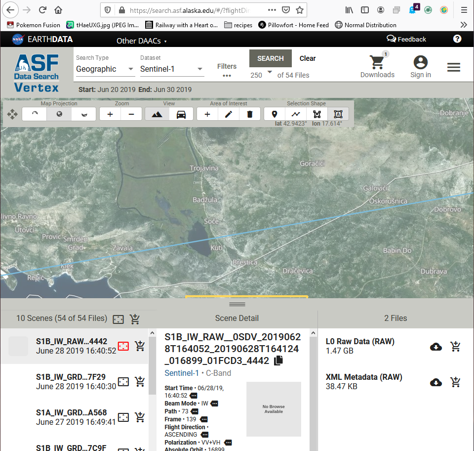
To acquire data, you will need to register an account with the Alaska Data Search, found here: https://search.asf.alaska.edu/#/?flightDirs. To do so, go to the link and select “sign in” then “Register”. Follow the instructions. This example uses the Bosnian and Herzegovinian and Croatian coastline. If desired, you can download several images and “stack” them. This process will be shown as well. Although SAR is purported to be "all weather", precipitation and sandstorms can adversely effect RADAR signals, so you may wish to check the weather of your AOI.

Find the area of interest that you wish to classify.

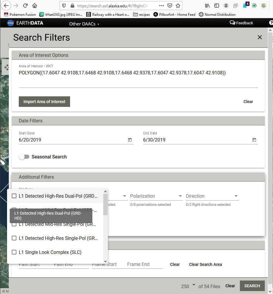
There is no need to use the exact image used in this tutorial, although the steps do require Sentinel 1 GRD format. GRD format can be input in the "Filters" window. If you do wish to use the image in the tutorial, parameters can be found below.

Example data Parameters

Search parameters:

Search type: Geographic

Dataset: Sentinel-1

Area of interest: POLYGON((17.6743 42.9283,18.3897 42.9283,18.3897 43.3711,17.6743 43.3711,17.6743 42.9283))

Start date:5/5/2019

End Date:6/13/2019

Under filters, select "L1 Detected High res Dual Pol(GRD)"

Frames: 140

Methods

The steps to complete the classification are as follows:

Set up your workspace by creating a folder on the drive you wish to work in. Save your images to this folder.

Open SNAP.

Import your data into SNAP using the “Import Product” button, and navigate to your working folder.

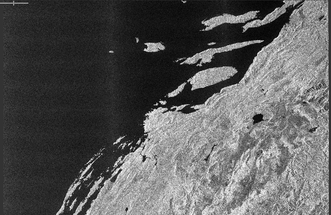
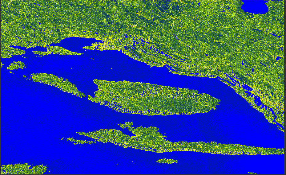
To get a feel for what your data looks like, double click the imported product to expand, then the “Bands” folder. Double click any band, and an image will appear of that band's backscatter imagery.

The band you open should look somewhat similar in composition to the image above.

As well, you can open the metadata folder in the product menu and examine characteristics relating to geographic location,satellite orbit, satellite incidence angle, and others. As you preprocess the image, this data will change.

Preprocessing

1.Subsetting

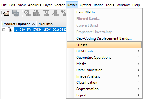
The next step will be to subset your image. Because of the time it takes to do unsupervised classification, you may wish to make a very small image.

Navigate to Raster ➔ Subset

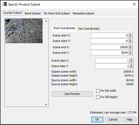
As shown in the images below, it is easiest to make a subset by dragging each side of the blue box on the left side of the Specified Product Subset window to the size you want, then selecting the middle and moving it to the desired area within the thumbnail image. Once you are satisfied, select the “OK” button.

If you wish to incorporate other images, you will need to copy either the Scene Start and End pixel coordinates, or the Geo-Coordinates, in order for your data to stack properly.

After you have completed the subset, right click the subset product in the Product Explorer pane and select "save product as" and save to your working directory. When repeating this step with other images, ensure that you copy the exact same values from either the Pixel Coordinates tab or Geo Coordinates tab used in your first subset. This guarantees all subsets have identical spatial extents and will stack correctly.

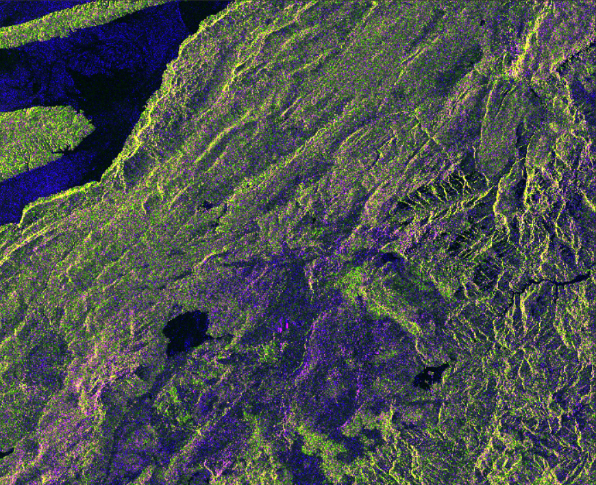
An RGB version of the tutorial subset image can be seen below. To view an RGB image, right click on the newly created subset and select "open RBG window".

Once this is complete, it is time to preprocess your image. Preprocessing is necessary because a raw SAR image can contain missing or incorrect geometric data.

Ensure you are writing to the working directory for all preprocessing and classification steps, and performing each step on each subsequent image.

2. Application of Orbit File

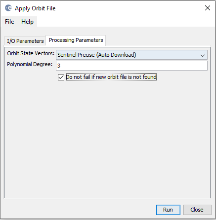
Over time, satellites can drift, and their orbit must be corrected. This can effect the recorded location of the image. To account for this orbital drift, SNAP can download precise satellite location information. To apply an orbit file, navigate to the Radar ➔ Apply Orbit File menu. The default of "Sentinel Precise" setting in the orbit state vectors dropdown menu does not need to be changed, but "Do not fail if new orbit file is not found" must be toggled.

3. Backscatter Conversion

Radiometric calibration takes into account factors such as the incidence angle, range spreading loss, antenna pattern gain and other sensor-specific characteristics of the image that impact backscatter intensity received by the sensor and normalizes it. Doing this allows for the comparison of SAR images from different dates, modes and sensors (Braun & Veci, n.d.). To note, radiometric calibration is not always necessary for qualitative analysis but it is essential when SAR data is used for quantitative analysis such as this (Calibration Operator, n.d.).

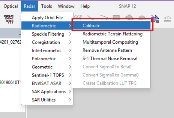
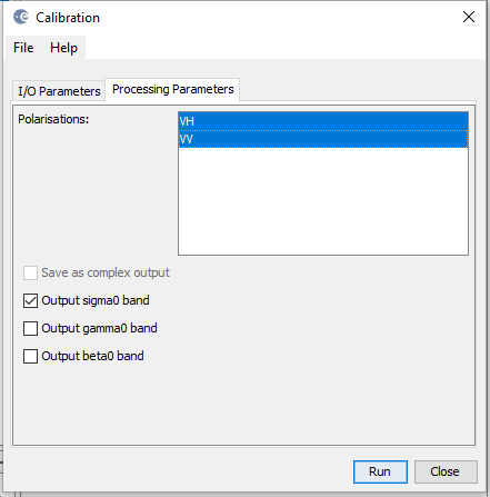
Navigate to the Radar ➔ Radiometric ➔ Calibrate menu.

Sentinel 1 supports different polarization modes which describe how the radar signal is transmitted and received. Select both VV (Vertical Transmit/Vertical Receive) and VH (Vertical Transmit/Horizontal Receive) polarization bands on the processing parameters tab and ensure the “sigma0” button is toggled.

Press Run.

VV signals are most sensitive to rough surface scattering which can be caused by bare soil or water while cross polarized data like VH are more sensitive to volume scattering from vegetation or forest canopies (Synthetic Aperture Radar (SAR), n.d.). Because they measure different types of scattering, using both together leads to a more accurate classification.

4. Speckle Filter

Speckle is a type of noise that appears in SAR images due to random constructive and destructive interference. Speckle filters can be used to suppress this noise, however, this is often at the cost of blurred features or reduced resolution (Braun & Veci, 2021). SNAP offers several filters including Lee, Refined Lee, Boxcar, Median and Gamma Map. The type and size of filter depend on the dataset and the intended application.

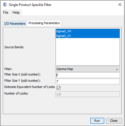
In this tutorial, we use a 7x7 Gamma Map filter as it offers several benefits when compared with other filters. Gamma Map models both speckle and scene reflectivity using a Bayesian approach, allowing it to reduce noise while maintaining radiometric characteristics of the image (Rana & Suryanarayana, 2019). It performs well in relatively homogeneous areas such as vegetation, water, or forested regions (Rana & Suryanarayana, 2019), and is also what Agriculture and Agri- Food Canada uses for image classification.

Navigate to the Radar ➔ Speckle Filtering ➔ Single Product Speckle Filter menu.

Select all processing parameter bands.

Find and select "Gamma Map" in the filter dropdown menu.

Type 7 in both the X and Y fields.

Press Run.

5. Geometric Correction

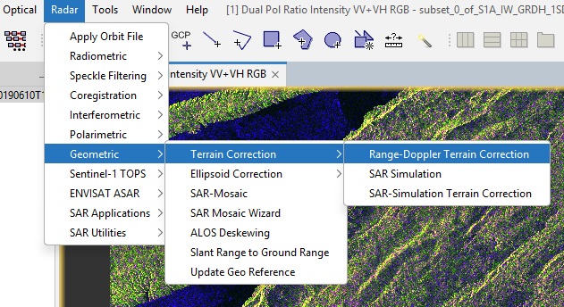
The purpose of terrain correction is to correct geometric distortions, such as foreshortening, layover and shadow, inherent in SAR imagery by using a Digital Elevation Model (DEM). This process geocodes the image from slant-range or ground range geometry into a map coordinate system (Braun & Veci, 2021). In this tutorial, we will be using the Range-Doppler Terrain Correction. This is the most widely used SAR imaging algorithm as it allows for motion compensation and provides a good balance between accuracy and processing efficiency (Sakr et al., 2023).

Navigate to the Radar ➔ Geometric ➔ Terrain Correction ➔ Range-Doppler Terrain Correction.

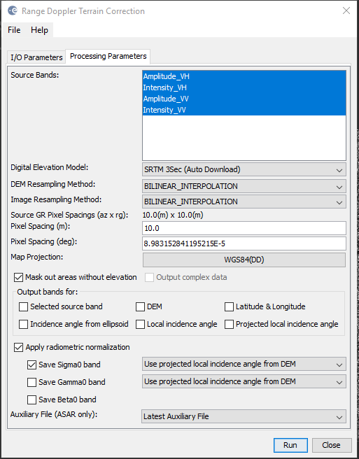
Under the "Processing Parameters" tab in the Range-Doppler Terrain Correction menu, select all source bands.

Toggle the "Apply radiometric normalization" button.

Leave all other values as default.

Press run.

If you only intend to run the classification on one image, skip the next step. If not, continue on to Coregistration.

6i. Coregistration

Coregistration aligns multiple SAR images to a reference image so that corresponding pixels represent the same geopositioning information and have the same dimensions. This step is necessary when stacking images from different dates or when combining datasets that are not already aligned, ensuring that pixel values can be compared or combined accurately. All images must also share the same projection system to work properly (Coregistration Tutorial, n.d.).

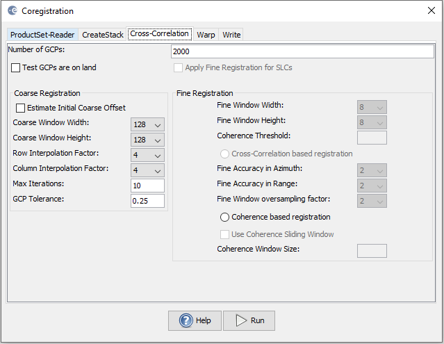
In SNAP, the coregistration operator uses the satellite orbits and image cross-correlation to match pixels with sub-pixel accuracy. The Cross-Correlation step refines the alignment between the reference and secondary images by measuring their offsets. The Warp step then resamples the secondary image using the calculated offsets so that it is geometrically aligned with the reference image (Coregistration, n.d.).

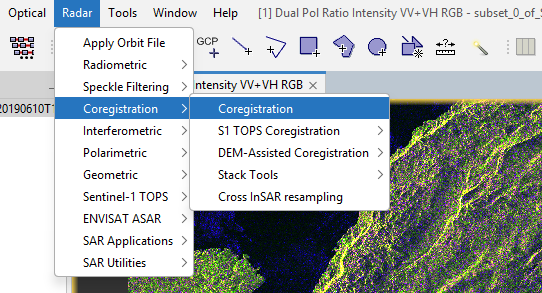
If you intend to run the classification on multiple images, you will need to "stack" them. To do this, navigate to the Radar ➔ Coregistration ➔ Coregistration menu.

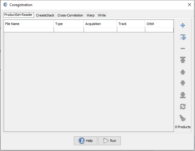
Add all your subset and preprocessed images by selecting either "add" (symbolized in 6.0 as a + sign), which will open a "Open Product" window, allowing you to navigate to your working folder and add the products of interest by selecting them and clicking "ok"; or "add opened" (symbolized as a + with a square background), which will add all open products to the ProductSet-Reader tab.

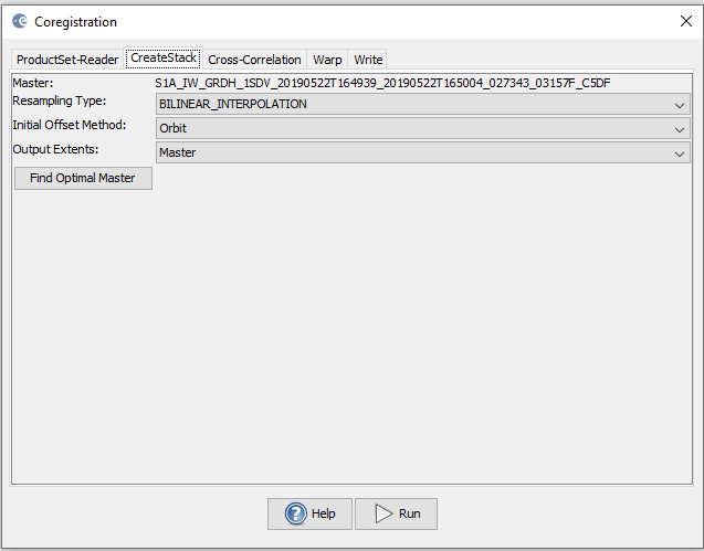
In the Coregistation window, select the CreateStack tab next, and select "Bilinear Interpolation" in the resampling type dropdown menu, and press "find Optimal Master".

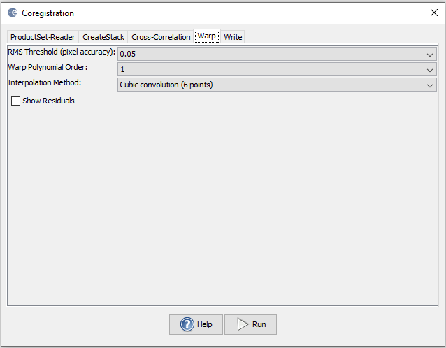
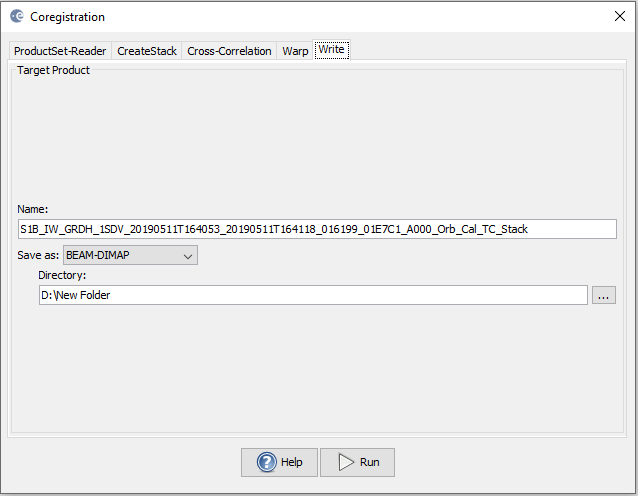
Do not make changes on the Cross-Correlation and Warp tabs. In the "Write" tab, save to your working directory.

Press Run.

6ii. Texture Analysis

Texture analysis is used to identify patterns in spatial distribution of pixel values and is an important characteristic for analyzing SAR imagery. It provides additional information about the structure of surfaces and helps distinguish between different land cover types, improving land-cover classification accuracy. The Grey Level Co-occurrence Matrix (GLCM) measures how often pairs of pixel values occur within a given distance and direction, which represents the probability of two grey levels appearing together (Texture Analysis, n.d.)

In SNAP, the GLCM operator computes second-order texture measures such as contrast, correlation, entropy and variance from a co-occurrence matrix over a specified window size (Texture Analysis, n.d.). We will use the Grey Level Co-occurrence Matrix texture analysis to generate texture bands. This can be a time consuming process, depending on the size of your image.

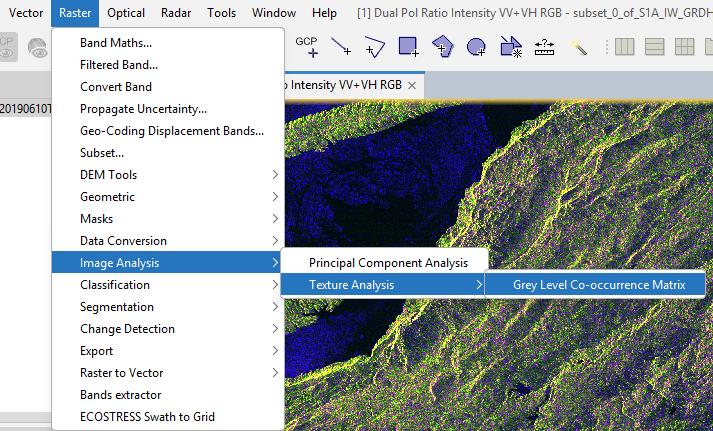
To apply the GLCM, navigate to Raster ➔ Image Analysis ➔ Texture Analysis ➔ Grey Level Co-occurrence Matrix.

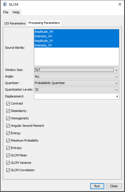
In the processing parameters tab, ensure all your bands are selected, and choose 7x7 in the windows dropdown menu. All other variables can remain as default.

Press Run.

The RGB result can be seen below.

Once the GLCM is complete, you can apply the classification.

7. Classification

To run the classification, navigate to the Raster ➔ Classification ➔ Unsupervised Classification ➔ K-Means menu.

Select the desired number of clusters; for this example on the Bosnian and Herzegovinian and Croatian coast, there were three clusters of interest, but depending on your area of interest there can be less or more. Both number of iterations and random seed can be left as their default values.

Select all the source band names you wish the classifier to use.

Press Run.

Note that this can be quite time consuming; however, if it has no progress after several hours, you may need to subset your image smaller, or reduce the amount of bands used for classification.

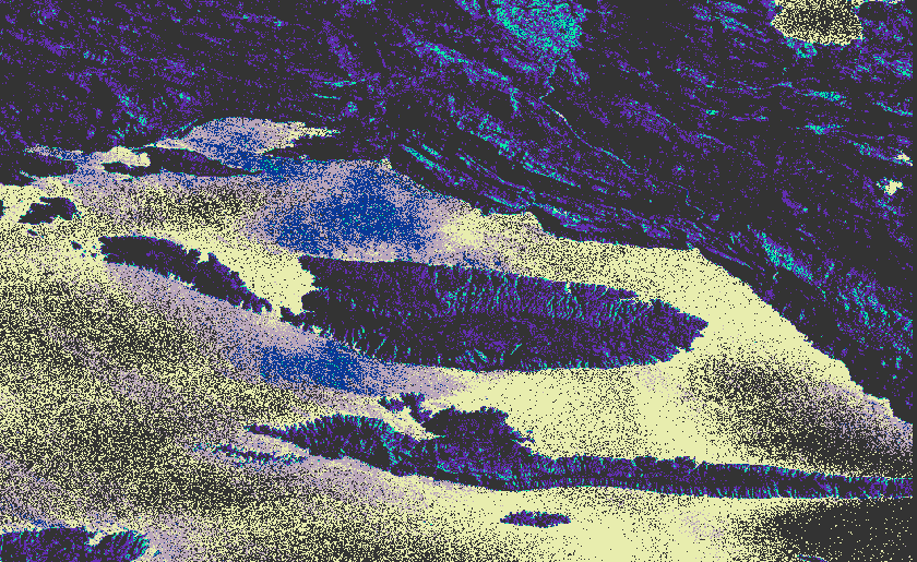
The result should look similar to the image below; however, colours may differ depending on your AOI and the cluster parameters.

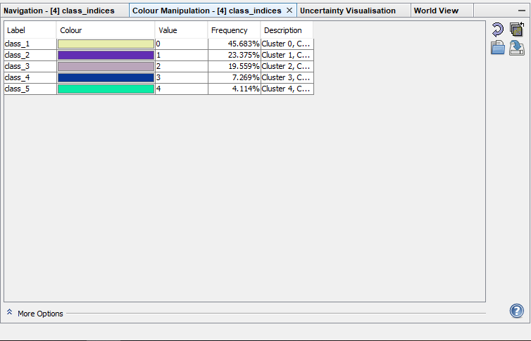
Colours and cluster names can be changed in the Colour Manipulation tab.

8. Validation

Note that, if this were an optical image, the water would all be a single colour. However, since SAR interacts with textures as well as water content, this will effect the classification. As well, there is the chance of miss-classified pixels.

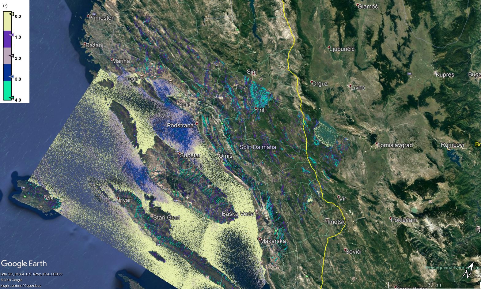
To validate the image, export as kml by right clicking the classified image and select "export view as Google Earth KMZ", and save.

If you open the kml file, it will open in Google Earth and you can visually assess the classes.

The image above shows that the teal is shallow water, yellow and dark blue are deeper water, and purple is vegetation. The grey "null" values are human infrastructure, such as buildings.

Conclusion and Citations

You can now preprocess GRD Sentinel 1 data, and perform an unsupervised K-means classification on dual-pol SAR imagery in SNAP.

Citations: Special Topics in Geomatics. Hosseini, M., & Mcnairn, H. (n.d.). Ottawa.