Leaflet Introduction with Multivariable Symbology
Contents
Introduction
Welcome to a beginner’s guide to using Leaflet, an open-source JavaScript library focused on web maps. In this tutorial, you will find the basics of downloading and setting up a Leaflet project and a deeper look at using web maps as a tool to visualize and analyse data using multivariable symbology. This tutorial will be implemented using the programming language of JavaScript, with the web implementation achieved via HTML. This tutorial was completed using Windows OS with specific reference to Windows functionality. Leaflet is compatible with all major Operating systems, but this tutorial provides specific instructions for Windows.
Download Leaflet & Data
Using Leaflet does not require the downloading of any software or libraries onto your local machine. The Leaflet library can be easily accessed for web mapping by simply calling a hosted version of Leaflet. This is what we will be doing for this tutorial, and the code required to make this connection will be explained in the next section.
Now onto the data, which we will be using for this tutorial. For this, we will be downloading weather station data from New Brunswick, Canada, for two reasons. The first is that the data is open and easily downloadable, and the second is that it has at least two variables which can be used for symbolising. It was downloaded from this page[1]. For this tutorial, the data used was from July and August of 2000. Once the date filter is set, scroll down to where it says “Data download format” and change it to GeoJSON. Then, click retrieve download links, and click the link that appears to download the data.
Creating the files
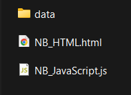
In a folder that can be easily accessed, create two text documents, one with the “.html” ending and the other with “.js”. In this same location, add a folder called “data” and move the downloaded GeoJSON into the data folder.
Open the .html and .js files in any text editor you like. The examples were created in VS Code for its auto-completion and formatting, making the coding experience beginner-friendly. The first thing to add will be the code provided by Leaflet, which allows for the connection to the library, the display of the map, and the connection to your JavaScript file.
HTML
In the head section of your file, you’ll need to copy the code below to provide default styling for the web map. Make sure to also include a style section of code where the map frame size will be defined
<head>
    <!-- Leflet CSS -->
        <link rel="stylesheet" href="https://unpkg.com/leaflet@1.9.4/dist/leaflet.css"
        integrity="sha256-p4NxAoJBhIIN+hmNHrzRCf9tD/miZyoHS5obTRR9BMY="
        crossorigin=""/>
    <style>
        #map { height: 600px; }
    </style>
</head>
Next in the body of your code, there will be three key sections added here at this point. The first section calls the leaflet script for the implementation into JavaScript, which is where all the functionality comes from this package. The second section defines and creates a generic box in html which is then populated by a map. The final section calls another script, but this time it is your own script where all the JavaScript code will be found. In this example, it is called “NB_JavaScript.js”.
<body>
    <script src="https://unpkg.com/leaflet@1.9.4/dist/leaflet.js"
        integrity="sha256-20nQCchB9co0qIjJZRGuk2/Z9VM+kNiyxNV1lvTlZBo="
        crossorigin=""></script>
    <div id="map"></div>
    <script src="NB_JavaScript.js"></script>
</body>
Altogether, the HTML file shows like this:
<head>
    <!-- Leflet CSS -->
        <link rel="stylesheet" href="https://unpkg.com/leaflet@1.9.4/dist/leaflet.css"
        integrity="sha256-p4NxAoJBhIIN+hmNHrzRCf9tD/miZyoHS5obTRR9BMY="
        crossorigin=""/>
    <style>
        #map { height: 600px; }
    </style>
</head>
<body>
    <script src="https://unpkg.com/leaflet@1.9.4/dist/leaflet.js"
        integrity="sha256-20nQCchB9co0qIjJZRGuk2/Z9VM+kNiyxNV1lvTlZBo="
        crossorigin=""></script>
    <div id="map"></div>
    <script src="NB_JavaScript.js"></script>
</body>
JavaScript
In your JavaScript file, this is where you will be manipulating the map and the data in the background. At the beginning of this code, it will simply differ the basemap, location of interest, and add the map to the empty frame created by the HTML file.
var map = L.map('map').setView([46.554, -66.136], 7);
L.tileLayer('https://tile.openstreetmap.org/{z}/{x}/{y}.png', {
maxZoom: 18,
attribution: '© <a href="http://www.openstreetmap.org/copyright">OpenStreetMap</a>'
}).addTo(map);
The first line simply creates the map variable and gives it an initial location using decimal degrees, and the defins the zoom level. The next section adds a basemap for the visualization of locations. For this, we will use OpenStreetMap (OSM)again because it is free and open (link osm here for more info). The “maxZoom” is a value that can be changed to restrict how far the user can zoom into the map. Feel free to play around with this value, with 0 being the most zoomed out and 19 being the limit for OSM tiles. The final line of code. is very simple; this completes the section and sends instructions based on the code above for how to display the map.
To check and see if everything is set up and working, navigate to your HTML file in your folders and open it to a web browser. This should open a new tab with a map which you can interact with, which is originally zoomed in on New Brunswick.
Creating a local server
Install Python 3 Before we connect the data to the web map, we must make the data readable by the web. This is most simply done by creating a local server. This will host the data securely and only locally on your network. For this toturial the simplest server is a Python server. If you do not have a version of Python 3 installed on you machin, go and download it [2].
To get the server up and running, navigate to the folder that contains your 2 scripts and the “data” folder
- In the blank space below the files, right-click
- Then click “Open in Terminal” which opens a command prompt for this folder
- Enter the text below and hit enter to start your local server
Python -m http.server
- When it starts, it should populate a new line with:
Serving HTTP on :: port 8000 (http://[::]:8000/) ...
- To access your files through your server, enter http://localhost:8000/ in your web browser
- Click on your HTML file to open your web map
Now that your file with both scripts and your data is being hosted, it can be called via the JavaScript file for visualization. The last thing to know is when you are done with the server, to close it, click into the terminal and type ctr+c.
Adding data
Now it’s time to connect the weather station so that its data can be seen in the map. This section of the tutorial will be written in the JavaScript file. To display this data, the GeoJSON found in the data folder needs to be opened in our file. Next, it will read through and find the coordinates of each station to use for presentation on the map. For this, we will also be separating the data into the two months now, so we have distinct layers for each month. The process of accomplishing this is separated into three distinct parts: linking to the data, making changes for visualization, and finally, the presentation.
Linking the data
This section of code is very simple to understand and to implement, but this is because of the previous setup, such as starting the server. The first line is extremely simple; it looks at the file that is being hosted, opens the “data” folder, and then opens the GeoJSON. The next two lines are relatively similar as they work together to make the data readable to the programming language and save it to a variable.
fetch("data/NB_2000_Aug_Jul.json")
  .then(response => response.json())
  .then(data => {
});
Changes for visualization
Working through the next section of code line by line, here’s what it does.
- Set a variable for the layer and a call to "data" which is where the data is stored
- Filters the data for any point that has the "Local data" equal to July 2000
- pointToLayer changes the default mark style so that it can be customized in future lines
- This creates a marker, which is a circle in the location of the latitude and longitude found in the data
- The rest are different options for customization of these point features
This section of code is repeated again for August.
const julyLayer = L.geoJSON(data, {
  filter: f => f.properties.LOCAL_DATE === "2000-07",
  pointToLayer: (feature, latlng) => {
    return L.circleMarker(latlng,{
        radius: 10,
        fillColor: "#ff0000ff",
        color: "#000",
        weight: 1,
        opacity: 1,
        fillOpacity: 0.8
    });
  },

});
Presentation
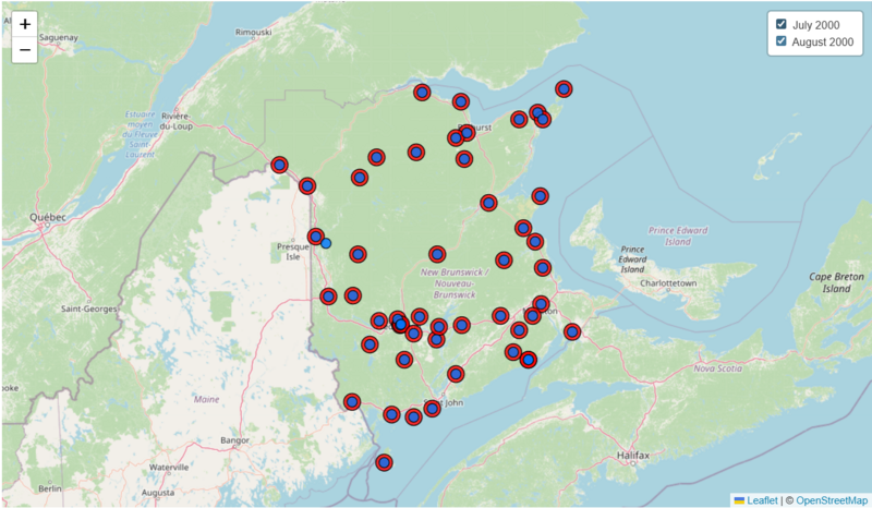
The first part creates the layer control tool, then adds the two layers with their names, which will appear in the control panel. This panel allows for the selection of the different layers. This is a great addition to any web map with more than one layer. The next line adds the panel to the map. Finaly both the layers are added to the map. Since the layers can be added through the control panel, just adding this step is not needed, but it is if you want them to appear from the first load of the map.
L.control.layers(null, {
  "July 2000": julyLayer,
  "August 2000": augustLayer
}).addTo(map);

julyLayer.addTo(map);
augustLayer.addTo(map);
Altogether
fetch("data/NB_2000_Aug_Jul.json")
  .then(response => response.json())
  .then(data => {
const julyLayer = L.geoJSON(data, {
  filter: f => f.properties.LOCAL_DATE === "2000-07",
  pointToLayer: (feature, latlng) => {
    return L.circleMarker(latlng,{
        radius: 10,
        fillColor: "#ff0000ff",
        color: "#000",
        weight: 1,
        opacity: 1,
        fillOpacity: 0.8
    });
  },
});
const augustLayer = L.geoJSON(data, {
  filter: f => f.properties.LOCAL_DATE === "2000-08",
  pointToLayer: (feature,latlng) => {
    return L.circleMarker(latlng,{
        radius: 6,
        fillColor: "#0077ffff",
        color: "#000",
        weight: 1,
        opacity: 1,
        fillOpacity: 0.8
    });
  },
});
L.control.layers(null, {
  "July 2000": julyLayer,
  "August 2000": augustLayer
}).addTo(map);
julyLayer.addTo(map);
augustLayer.addTo(map);
});
Changing the symbology
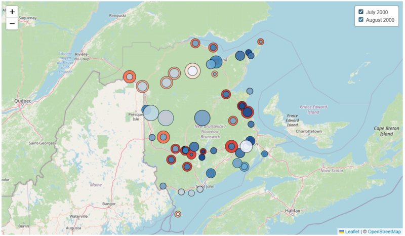
This is the main difference between this tutorial and others, as this is where we can begin to create the comparison between different layers. In this tutorial, we will be using average temperature and total rainfall to change the colour and size of the circle, respectively. By applying this to both months, it allows for a visual comparison of values between months. To accomplish this, four functions will be made. Two functions deal with the colours for temperature, one deals with the size of the circles, and the last function applies the correct colour scheme for either month and adds this to the styling of the circles. When adding the functions into your code, it is important to note that this should be placed at the beginning of the document, only behind the section which sets the location and basemap.
For the colour and temperature functions, these are practical, they same with the only difference being the values they return. To accomplish this, the function will take one variable as an input, which is used to compare against various values to sort each station into groups of either temperature or total rainfall.
function tempColour_july(t) {
  return t >= 19 ? "#a50f15" :
           t >= 18 ? "#de2d26" :
           t >= 17 ? "#fb6a4a" :
           t >= 16 ? "#fcae91" :
           "#fee5d9" ;
}
function tempColour_august(t) {
  return t >= 19 ? "#08519c" :
           t >= 18 ? "#3182bd" :
           t >= 17 ? "#6baed6" :
           t >= 16 ? "#bdd7e7" :
           "#eff3ff" ;
}
function precipSize(p) {
    return p >= 125 ? 20 :
           p >= 100 ? 16 :
           p >= 75 ? 12 :
           p >= 50 ? 8  :
                     4;
}
In the JavaScript code, this is accomplished using “?” which says if the comparison beforehand is Ture then set the value to what follows the question mark. If the condition is false, it moves to the next comparison.
The last function puts all of this together into a function which can be easily called when adding the data to the map.
function styleStations(feature) {
  const temp = feature.properties.MEAN_TEMPERATURE;
  const rain = feature.properties.TOTAL_PRECIPITATION;
  const month = feature.properties.LOCAL_DATE;
  let colour;
  if (month === "2000-07") {
    colour = tempColour_july(temp);
  } else {
    colour = tempColour_august(temp);
  }
  return{
    radius: precipSize(rain),
    fillColor: colour,
    color: "black",
    fillOpacity: 0.85,
    weight: 0.75
  };
}
Again, this function takes a single argument, which will be each individual station’s data. The next three lines simple creates variables for where the program can find the temperature, rainfall, and date information in the data. The variable for which months' colour is also created here. Next comes the if statement, which determines which month the data is from and assigns it the correct colour scheme. It does this by first checking if the month is July; if this is True, then it sets “colour” to the July colour scheme using the previously created function. If the month is not July, it does the same thing, but for August. The final section states what this function will give back as a return. For this, it uses the same formatting seen when the data was originally entered, except this time, some of our values are variables and function calls. For example, radius calls the function created to alter the size of the circle.
Now we need to use this function to actually change how the data will be displayed. To do this will require minor alterations to the current code. Simply remove the section which sets the parameters for the circles and add the call to the last function created with “feature” entered as the argument. Make sure to do this for both months.
//Old code
const julyLayer = L.geoJSON(data, {
  filter: f => f.properties.LOCAL_DATE === "2000-07",
  pointToLayer: (feature, latlng) => {
    return L.circleMarker(latlng,{
        //REMOVE THIS
        radius: 10,
        fillColor: "#ff0000ff",
        color: "#000",
        weight: 1,
        opacity: 1,
        fillOpacity: 0.8
        //until here

const julyLayer = L.geoJSON(data, {
  filter: f => f.properties.LOCAL_DATE === "2000-07",
  pointToLayer: (feature, latlng) => {
    return L.circleMarker(latlng,styleStations(feature)); // added this part at the end
  },
});
And that’s it! You should now see a web map with weather stations that have different colours and sizes based on two different climate variables.


