Emergency Shelter Allocation Evaluation
Contents
Introduction
 FACT: Hawaii is the State most at risk of Tsunami conditions, Getting about one per year, a highly damaging one every 7 years. The biggest tsunami that occurred in Hawaii happened in 1946 when the coast of Hilo was hit with 30 ft waves at 500 mph, 170 fatalities. Click here for more facts of Tsunami Danger.

This project demonstrates how to make a spatial decision that determines the best use of monetary resources when further developing the emergency preparedness framework of a community. Spatial allocation decisions often can not be made most efficiently with consideration of only an independent variable, and scenarios realistically exist as multi-criteria based. This tutorial will demonstrate how this evaluation can be carried out using only Free and Open-Source Software(FOSS), particularly using the Quantum GIS (1.8.0) package and the GRASS Plugin.
Particularly, the scenario that outlines what the objectives are for this tutorial involve the expansion of Emergency Shelters in Hawaii pertaining to the emergency of a Tsunami event. The funding for this expansion has specific criteria which is as follows:
- Funds must be concentrated to the area of highest risk to large waves within the State.
- Shelter Location must be far away from Evacuation Land.
- Shelter Location must be in area of highest population density.
- Shelter Location must be far away from existing Shelters.
This tutorial is directed towards someone who has a minimal or basic understanding of GIS. The processes outlined throughout this tutorial may also be applicable in understanding gaps of public safety as a community evolves, or something as simple as determining the best location for a business expansion. The variety of applications are extremely widespread.
Data Collection
For this specific scenario, it was necessary to collect a variety of shapefiles (vector data) that are freely available online. There is a variety of online databases that have appropriate files with access to download freely. Sources of data very much depend on your geographical location and the government availability of free files.In this particular case the data was gathered from a catalog provided by the Hawaii State Government and U.S Census Bureau. Table 1. provides a specific breakdown of where each file was found and the adequacy of it.
| Shapefile Name | Format | Data Source | Description |
|---|---|---|---|
| Tsunami Evacuation Zones | Vector Polygon - Preliminary Analysis/Final Anaysis File | Hawaii State Office of Planning | High risk area to Tsunami impact. |
| Tsunami Wave Heights | Vector Point - Preliminary Analysis File | Hawaii State Office of Planning | Locations of large wave events along the coast, attributes include year by year breakdown of events. |
| Emergency Shelters | Vector Points | Hawaii State Office of Planning | Locations of Shelters, and individual capacity. |
| Census Tracts | Vector Polygon | U.S Census Bureau | Total Population by tract, 2009 TIGER/Line Shapefiles for: Hawaii |
Setup
As mentioned within the introduction Quantum GIS(QGIS) version 1.8.0 is used to carry out this analysis, and within this platform the GRASS Plugin is also used in combination with QGIS tools. The following three sections will provide specific instructions as to how to download the necessary software and the appropriate set up to begin your project.
Install QGIS
If you don't already have the appropriate software downloaded to your computer, Click here to do so according to your running platform of your computer. I used Windows 1.1 Standalone Installer, and had no problems. Along with this download is the GRASS package that will allow you to add the GRASS plugin once you are in QGIS, requiring no additional download for this plugin.
Install GRASS Plugin
From this point forward through the tutorial it is assumed you have QGIS open. Having the GRASS plugin installed within your project allows for access to a wide variety of additional tools that are extremely useful, as you will see throughout this tutorial. The following steps will direct you to successfully loading the GRASS plugin.
- Click Plugins tab ⇒ Click Manage Plugins ⇒ This will open up QGIS Plugin Manager Window
- In filter type GRASS, and ensure there is an X in the box ⇒ click OK.
- Click Plugins tab ⇒ GRASS tab will now appear ⇒ Expand the list of tools ⇒ Click 'New Mapset'
- Click Browse to find destination folder NOTE: you must have a destination folder already in Windows Explorer ⇒ Click Next,
- Create new location (Named mine Project) ⇒ Click Next.
- Define your projection. This can be found within the metadata of your shapefiles, or on the site from which you downloaded the data ⇒ Click Next.
- Define GRASS region ⇒ I selected USA, as it seemed most appropriate ⇒ Click Next.
- Name your mapset (Named mine Hawaii)⇒ Click Next.
- Click Finish, mapset has now been created.
- Go to the Plugins tab ⇒ Click GRASS ⇒ Click Open Mapset ⇒ Select what you have just created and now your work will be within this mapset.
Setup Workspace
Before starting anything further it is important to save your workspace.
- Click File tab ⇒ Click 'Save Project As' ⇒ save it alongside your other data.
- Continue to save workspace ongoing.
Then you can load your shapefiles into your workspace (Only Vectors to work with):
- Click the 'Add Vectors' button at the top left of the screen.
- Leave the 'Source Type' as File, and Encoding as System (default).
- Browse to location you saved your data and click a file (Press Ctrl on keyboard to select many at once)⇒ Click Open ⇒ Your data will now be visible and the layers are a part of the table of contents on the left hand side of the window.
Preliminary Analysis
Initially it is necessary in this particular instance to perform a preliminary analysis. This will narrow down exactly what region of Hawaii is most vulnerable to Tsunami activity.
Deciding Area of Interest
The shapefiles used for this process were Tsunami wave event recording points and Evacuation Land polygons, outlined in Table.1. The area of interest was determined based on the quantitative attributes within each file. The following section will outline the process of creating an output that would assist in deciding what the most vulnerable area is, resulting in our specific area of interest.
Quantitative Map Output
Exploring the attributes is majorly helpful in deciding how to manage the data available. That is the first step I took. To view the attributes please follow these outlined steps:
- After adding your data to the table of contents, you will now be able to view all necessary layers.
- Right click the title of your layer (file name) which will open a menu ⇒ click 'Open Attribute Table'
- Here you will be able to view the columns of data.
I chose the Wave Heights layer to explore first. It had a column for each significant year of high waves, showing the highest recording of that year for each storm location. I then thought it would be appropriate to quantify these values spatially. To do so it was necessary to edit the attribute table, and add an additional column to calculate the total significant recordings. The following steps outline how I processed this information:
- Within the Attribute table window Click the 'Toggle Editing Mode' button
 ⇒ Click 'Add Column' button
- Type in an appropriate name, and keep the Type as Whole Number ⇒ click OK.
- Click the 'Open Field Calculator' button
 ⇒ Make sure X is in box beside update existing field.
 - Select Field to edit in drop down menu ⇒ selecting field just created. NOTE: There is an option to the left of the calculator to add field at the same time as calculating data, but I have broken this down into separate steps.
- Create an expression. The expression used here is very simple. I selected fields that had wave height information in them and added them together to create a total.
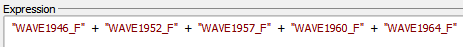
The resulting column looked like this:
- Click the 'Save Edits' button within the Attribute table window.
- Toggle off the 'Toggle Editing Mode' button ⇒ Close the attribute table window.
Secondly, I explored the Evacuation Land shapefile attributes. It's attributes were much more simple and already had a column signifying the AREA of each parcel of Evacuation Land. The parcel with the largest area was determined as most significant. This brings us to the cartographic symbology process. This is relatively easy, the following outlining the specific steps.
Symbolizing the Evacuation Land layer:
- Right click the layer name ⇒ Click 'Properties'
- Click the 'Style' tab ⇒ where it says single symbol click the drop down menu and select 'Graduated'.
- Select column to symbolize, in this case it was AREA ⇒ choose a colour ramp, decide the number of classes appropriate (in this case 6), and type of classification (in this case equal interval).
- Click 'Classify' at the bottom left of the window ⇒ then 'Apply' and 'OK'
You should now see the layer symbolized, and the legend can be seen by expanding the layer in the table of contents.
Symbolizing the Tsunami Wave Height Event layer:
- Right click the layer name ⇒ Click 'Properties'
- Click the 'Style' tab ⇒ where it says single symbol click the drop down menu and select 'Graduated'.
- Select column to symbolize, in this case it was WaveHeightTotal ⇒ choose a colour ramp, decide the number of classes appropriate (in this case 4), and type of classification (in this case equal interval).
- Click 'Classify' at the bottom left of the window ⇒ then 'Apply' and 'OK'
You should now see the layer symbolized, and the legend can be seen by expanding the layer in the table of contents.
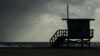
The following image shows the most vulnerable coastline area in Hawaii (by a very long shot). Assume the NW side of the area to be ocean, and the SE side to be the inland. 
This map quantitatively shows the information edited earlier. However, the polygons of the Evacuation Land is somewhat determined based on the population of that area (county/metropolitan area) rather than based on a terrain analysis, which could be considered an inconsistency and tough to base an accurate decision off of it independently. This brings in the importance of the Wave Height Total layer. It shows a remarkable number of incidents, all of which are the highest or second highest events in the state. Therefore, this area of Hilo City was determined as the area of interest for this project, despite some inconsistencies within the data. For the sake of this being a precautionary preliminary step this is a pretty good method of narrowing down a area of interest (AOI). Further analysis could be done by finding the historical records of the state, and statistically analyzing the information and create your own vector layer accordingly.
Data Processing
This section involves preliminary editing that narrows the data collected for the entire state down to just the AOI of Hilo. These stages will bring simplicity to the later stages of this project, and have all the files in the exact formats necessary to carry out this analysis.
Please note: altering the projection was not necessary in this project, and therefore not included in this tutorial. If this is the situation for your data please click here for methods of changing projection.
Clipping to AOI
Clipping is the process of creating a new vector file that include only the data required for the very specific area of interest. The input features are extracted and made into an individual vector file. In this case Emergency Shelters, Evacuation Land and the Census Tracts data is needed to be clipped (Wave Heights not useful beyond preliminary analysis). The following will outline the steps necessary to complete a Clip.
- Select the 'Select by single feature' icon, and this will now allow your mouse to select the features that are included in your study area. You can also use 'Select by Rectangle', but often the irregularity of study areas causes for sections to be selected that aren't necessarily applicable. You can also select through the attribute table, there are many ways about going to do this.
- Once you have all the data within AOI selected ⇒ Click 'Vector' tab at the top of the QGIS window ⇒ Click 'Geoprocessing Tools' ⇒ Click 'Clip'
- Choose your input vector layer to be clipped ⇒ Ensure there is an X in the box that says 'Use only selected features'.
- Use Census Tracts Data to be the clip layer (extends beyond all other necessary data in this case) ⇒ Ensure there is an X in the box that says 'Use only selected features'.
- Name an output name in the appropriate directory by clicking 'browse' ⇒ Click 'OK'
- Repeat the last three steps again for all vectors that need to be clipped, in this case this was done for Emergency Shelters (output named ES.shp) and Evacuation Land (output named EL.shp)
After Clipping was complete, my data looked like this:

Dissolve AOI
This stage of data processing is necessary because after using the proximity tool within the methods section, the created output from this step will be used as a mask to clip that raster file to this extent. Dissolving simply means taking a vector file with multiparts (in this case multiple polygons) and making it one uniform polygon. In this project, a dissolve was performed on the Census Tract polygon vector file. The following steps outlines how this was done.
- Once you have all the data within AOI selected ⇒ Click 'Vector' tab at the top of the QGIS window ⇒ Click 'Geoprocessing Tools' ⇒ Click 'Dissolve'
- Input Census Tracts layer ⇒ dissolve the AREA field ⇒ name an output file and place it in appropriate directory ⇒ Click 'OK'

The above image shows the before and after of the dissolve tool.
Attribute table editing
To turn on the capability of editing your attributes please follow these steps:
- Right click the title of your layer (file name)in the table of contents which will open a menu ⇒ click 'Open Attribute Table' ⇒ Here you will be able to view the columns of data.
- Within the Attribute table window Click the 'Toggle Editing Mode' button