Georeferencing Raster Imagery in QGIS using Vector Data

Introduction

QGIS

QGIS [[1]]

QGIS, previously known as Quantum GIS, was initially created by the Open Source Geospatial foundation in 2007 and is maintained by the QGIS Development Team. The software is written in C++ language. The software integrates many plugins that are written in either C++ or Python. SQLite, GDAL, GRASS GIS, PostGIS and PostgreSQL provide users with access to different data formats. QGIS is cross-platform and is able to operate on Mac OS X, Linux, UNIX and Microsoft Windows. QGIS is available in multilingual formats and is licenced under GNU GPL (OSGeo) http://www.qgis.org/en/site/about/index.html.

QGIS can be used in conjunction with other open source GIS software packages such as PostGIS, GRASS and MapServer in order to extend the software’s capabilities. Users have access to Python plugins and plugins that are able to geocode using the Google Geocode API as well as an array of geoprocessing tools that are similar to those found in the well-known software package ArcGIS. QGIS is free open-source geographic information system (GIS) software that provides users with the ability to view, edit and analyse data. Users are able to generate maps using a variety of map layers using different projections. QGIS is compatible with both vector and raster data as well as geodatabases.

Georeferencing

Geo-referencing in GIS allows the user to use a known coordinate system to align geospatial data so that it may be viewed, queried or analyzed with other geospatial data. This process involves manipulating the data through shifting, scaling, rotating or skewing in order to align the datasets.

Satellite imagery can be affected by geometric distortions as a consequence of sensor geometry, inconsistency in the scanner or platform, earth rotation or earth curvature. These issues can be corrected by referencing the imagery to existing maps. Since satellite imagery and aerial photographs do not contain reference information to a location when in their original format. In order to use this information in combination with other geospatial datasets it is necessary to correct the imagery so that it has a similar resolution and projection as the data you wish to work with.[3]

Acquiring Data

Geospatial data can be downloaded from Geobase [4] or the Geoconnections Discovery Portal online [5]

The files used for this example include the following:

Table 1. Data Used in Geo-referencing Aerial Photography and Satellite Imagery

Data Used	Data Format	Data Source
Rail	Vector Polygon	Layer: Rail, 2010 / Producer: Carleton University Construction Services
Carleton Boundary	Vector Polygon	Layer: Carleton Boundary, 2010 / Producer: Carleton University Construction Services
Canal	Vector Polygon	Layer: Canal, 2010 / Producer: Carleton University Construction Services
Buildings	Vector Polygon	Layer: Buildings, 2010 / Producer: Carleton University Construction Services
Rideau River	Vector Polygon	Layer: Rideau River, 2010 / Producer: Carleton University Construction Services
Roads	Vector Polygon	Layer:Roads, 2010 / Producer: Carleton University Construction Services
Satellite Imagery	Portable Network Graphics (PNG)	Layer: Carleton University Campus, 2010 / Producer: Digital Globe (Google)

Disclaimer

It is highly recommended that these steps are followed in the order that they are written in order to avoid confusion.

Installation

• QGIS can be downloaded from the following link [6]

Figure 1. Download [[2]].

• Choose the latest version of QGIS
• Follow along with the Installation Wizard and save QGIS to the appropriate directory
• Once the installation process is complete, QGIS can be run.

Starting QGIS

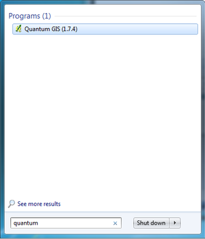
• Open QGIS from your start menu in order to run the software.

Figure 2. Opening QGIS.

Figure 3. QGIS Interface.

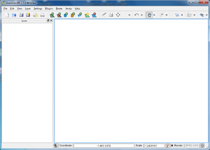
• Once the software is initiated, the QGIS window will appear.

Adding Geospatial Data in QGIS

Vector Data

• To add vector data into QGIS navigate to the toolbar situated at the top of the window, as demonstrated in Figure 4.
  

  Figure 4. Toolbar
• Select the vector icon.

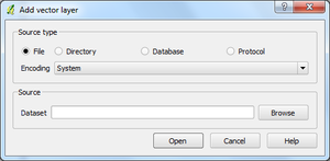
• A window will appear that prompts you to choose your file.
  
• Toggle on the appropriate source type and set the coding option using the drop down menu.
• Next, browse to the source of your vector file by clicking the Browse button on the window as seen in Figure 6.

Figure 6. Vector File Window.

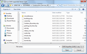
*This will bring up the search window.

• Navigate to your file and select Open.
  
  

Figure 7. Browsing Files.

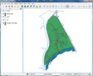
• Your file will appear in the Table of Contents (TOC) and is drawn in the white space in the QGIS window.

Figure 8. Vector Layers.

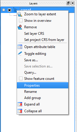
• To look at properties associated with each file and change symbology, right-click on the appropriate file in the table of contents.

‎

Figure 9. Properties.

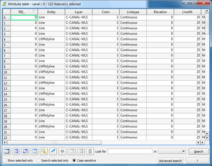
• To view data associated with your vector file, select Open Attribute Table.

Figure 10. Attribute Table Values'.

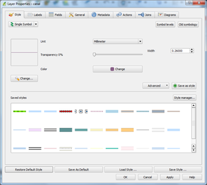
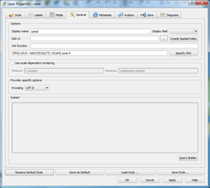
• A window will open that will provide users with a variety of options associate with the file. Figure 11. Properties and Symbology, shows the symbology of the file. Users are able to change how their data is represented using this tab. Additional tabs such as Labels, Fields, General, Metadata, Actions, Joins and Diagram allow users to manipulate their data as is appropriate.

Figure 11. Properties and Symbology'.

• Select the General tab in order to view the file projection and name.
  This is become particularly useful whenever georeferencing a raster file to match the projection of your vector layers.

Figure 12. Properties.

Raster Data

• To add a raster file into QGIS navigate to the toolbar at the top of the window and select the raster icon.
• Follow the steps provided for adding a vector file.

Accessing a Plugin

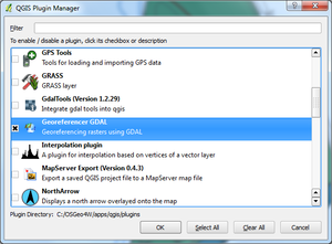
• To access the plugins available in QGIS navigate to the main toolbar and under Plugins select Manage Plugins.

Figure 13. Plugins Toolbar.

• A window will open providing you with several options for plugins. Scroll through them until you come across Georeferencer DGAL.
• Toggle the Georeferencer on and select OK

Figure 14. Available Plugins.

Using Georeferencer DGAL

The Georeferencer allows you to reference rasters to geographic coordinates or projections by creating a new GeoTiff file by adding a world file to the existing raster image. To reference a raster you are to locate points on the image that you can accurately identify their coordinates. X and Y coordinates can be Degrees Minutes Seconds (dd mm ss.ss), Decimal Degrees (dd.dd) or projected coordinates (mmmm.mm) depending on your data.

Opening the Georeferencer

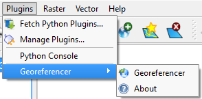
• Navigate to the main toolbar, and select Plugins. A drop down menu will appear with the Georeferencer now available to you.
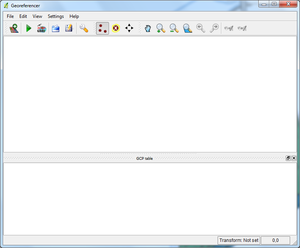
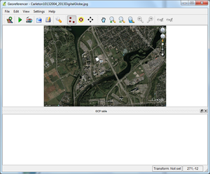
• The Georeferencer window will appear and you will be able to add the file you wish to georeference.

Figure 15. Georeferencer Plugin.

Adding a Raster

• To georeference your image, you must first add it into the georeferencing window.

Figure 16. Georeferencer Toolbar.

• Navigate to the main toolbar for the georeferencer and select the raster icon.
• Follow the steps provided for adding a vector file to navigate to and add the appropriate raster file.

Figure 17. Georeferencer Toolbar.

• Once your image has been added, it will appear in the centre of the georeferencer screen.

Figure 18. Raster Image'.

Adding Control Points

If you already have control points saved, you can load the file by selecting the Load Points icon Otherwise… Select the add control point icon .

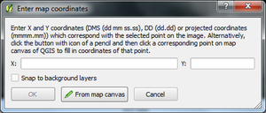
• A window will appear prompting you to add the coordinates of the point, or find it on the referenced file within the main window of QGIS.
• If you know the coordinates, enter them. Otherwise select From Map Canvas

Figure 19. Adding a Point.

• To delete a point, select the Delete Point icon
• You can move points by selecting the Move Points icon on the toolbar.

Zooming In and Out

• To zoom in on the image in the georeferencer window select the Zoom In icon.
• To zoom out on the image in the georeferencer window select the Zoom Out icon.
• To move around the image, select the Pan icon

Points Table

• The points which you have placed on your map image will appear below the raster image in the window.
• To save your points select the Save Points icon on the toolbar.
• This will save your points to an .aux.xml file for later viewing, or to add back into the Georeferencer.
• If the residuals are high for some of your points, you should go back and move the point to be more accurate.

Transformation Settings

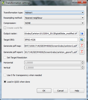
To access the transformation settings navigate to the toolbar on the Georeferencer and select the Transformation Settings icon.
After adding the Geographic Control Points (GCPs) you will need to define the settings for the georeferencing procedure.

• Depending on how many points you have added to your image you may want to choose different transformation algorithms for your image.

Transformation Type

Choose an appropriate transformation type.

• The transformation types available to you include:
  • Linear: This is used to generate a world-file that will be different from the other algorithms available because it does not actually transform your image. This probably won't be the best option if you are using scanned imagery.
  • Helmert: This transformation will run simple scaling and rotation transformations.
  • Polynomial Algorithms: These will match source and destination control points. The 2^nd order polynomial transformation allows for some curvature in your transformation. Using a 1^st order polynomial transformation (affine) will perserve collinearity and will only permit scaling, translation and rotation on the image.
  • Thin Plate Spline: This transformation is able to introduce local deformations in the data. This is good if the original image being georeferenced is of poor quality.
  • Projective: The projective transformation is a linear rotation and translation of coordinates.

Defining the Resampling Method

• Select one of the resampling method options by clicking on the drop down list. Your choice will vary depending on the objectives of your task.
• Choose one of the following options:
  • Nearest neighbour
  • Linear
  • Cubic
  • Cubic Spline
  • Lanczos

Compression

• Select the type of compression you wish to occur on your image.
• The options include:
  • NONE
  • LZW
  • PACKBITS
  • DEFLATE
    

Output Raster

• Select the location for the output file by selecting the Output Raster icon and navigating to the appropriate folder.
  

Target Spatial Reference System (SRS)

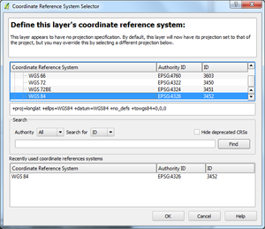
• Choose the target coordinate system for your raster image by clicking the SRS icon [[7]]
  
• A window will appear prompting you to choose a coordinate system for your image.

Generating a pdf map and report

• To save a map or report to disk as a .pdf file, select the .pdf document icon next to Generate pdf map and/or Generate pdf report.
• Navigate to the appropriate directory to save your files.

Figure 23. "pdf Output from Georeferencing"

Set Target Resolution

Toggle on Set Target Resolution to set the pixel resolution for your output raster.

Additional Options

• Toggle on Use 0 for transparency when needed to make areas with the value of 0 transparent.
• Toggle on Load in QGIS when done to add the image into QGIS as a layer whenever the georeferencing process is complete.
• Toggle on Create world file for linear transformations.

Select OK when complete.

Running the Georeferencer

Once all of the GCPs have been added and the Transformation Settings have been selected you can now georeference your raster image.

• Select the Start Georeferencing icon on the main toolbar.
• This will create a new georeferenced image.

Georeferenced Raster

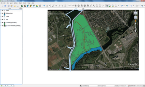
QGIS will prompt you to add the new georeferenced raster into your map document. The file will appear in the Table of Contents. Move your layers so that the vector polygon layers appear on top of the raster image.

Figure 24. "Georeferenced Raster with Vector File Overlay"

Map Design

To produce a map layout additional features can be added to your map document.

Adding a Scale bar

• To add a scale bar navigate to the main toolbar in QGIS and select Plugins

Figure 25. "Toolbar in QGIS"

• Select Manage Plugins
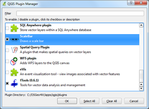
• A window will appear prompting you to choose a plugin. Toggle on Scale Bar.

Figure 26. "Scale Bar Plugin"

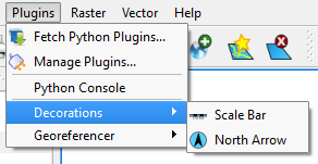
• Now navigate to the main toolbar in QGIS and select Plugins, a list of options will appear in a drop down menu.
• Select Decorations and then Scale Bar.

Figure 27. "Scale Bar Tool"

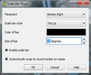
• A window will appear with options for the toolbar.
• Choose the desirable options and then click OK

Figure 28. "Scale Bar Options"

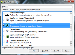
Adding a North Arrow

• Navigate to the main toolbar in QGIS by following the instructions above.
• Toggle on the NorthArrow plugin.
  

Figure 29. "North Arrow Plugin"

• Select OK and then navigate to the main toolbar, select Plugins and use the drop down menu to navigate to Decorations.
• Select North Arrow
• A north arrow will be added to your map document.

Terms

GNU GPL

The GNU General Public Licence is a widely used free software license that allows users of the software the liberty to use, study, share and modify the software. [8]

C++

C++ Language is an open ISO-Standardized language and is a compiled language. It supports both manifact and inferred typing as well as both static and dynamic type checking. It is able to run on many different platforms and has a large support library for help. [9]

Python

Python programming language runs on a variety of platforms and is free to use since it is an OSI-approved open source license. [10]

Vector Data

Vector Data is a coordinate-based representation of geographic features by way of points, lines and polygons. An individual point feature is represented as a singular point pair whereas ordered lists of vertices represent polygon and lines. Attributes as associated with each feature in vector data. [11].

Raster Data

Raster data represents space as a grouping of equally sized cells that are organised in rows and columns that are made up of singular or multiple bands. Each of these cells contains both an attribute value and coordinates. Similar cells represent the same type of feature and coordinates are stored in the ordering of the matrix. Rasters can be digital aerial photographics, satellite imagery, digital pictures or scanned map and can be either thematic (discrete) or continuous [12]