Slope Analysis using Quantum GIS Processing Toolbox

Getting Started

Launching QGIS 2.2

When the installation process has finished, an icon should appear on your desktop similar to the one shown below.

Double-click on that icon and QGIS 2.2 will display on your screen.

Setting Project Coordinate Reference System (CRS)

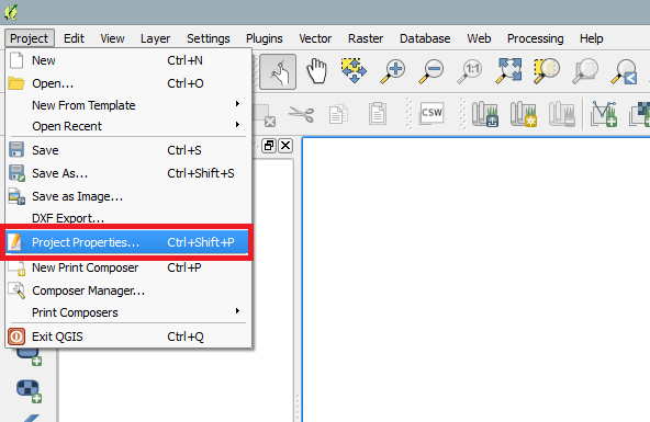
Following the launch of QGIS 2.2, navigate to the top menu bar, select Project, Project Properties, then CRS.

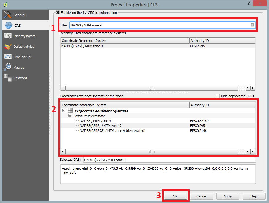
Make sure that Enable 'on the fly' CRS transformation is checked (1). Once enabled, filter search (2) NAD83 / MTM zone 9 and select NAD83(CSRS) / MTM zone 9 under the Coordinate system reference systems of the world. When finished select (3) OK.

Adding Vector Shapefiles

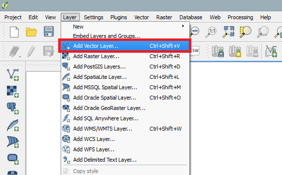
Adding the Carp shapefiles or your desired shapefiles requires navigating to the menu bar, select Layer and Add Vector File...'.

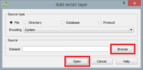
A dialogue box will open asking for the destination where the shapefiles are located. Select Browse and navigate to the folder where you saved the shapefiles. Click Open.

Processing Toolbox

Open Processing Toolbox

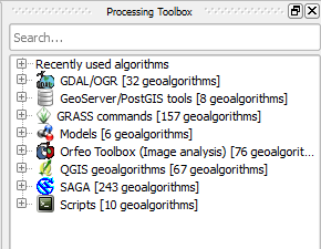
If the Processing Toolbox is not already displayed on the right side of the QGIS 2.2 window, under Processing in the menu bar, select Toolbox.

This will display the Process Toolbox on the right side of the screen.

Creating a model using Graphical modeler

To create a model workflow navigate to the menu bar, under Processing, select Graphical modeler.

Once the modeler window has opened, you can begin to create the desired workflow. For this particular tutorial, the Carp shapefiles will be used to create a slope analysis workflow.

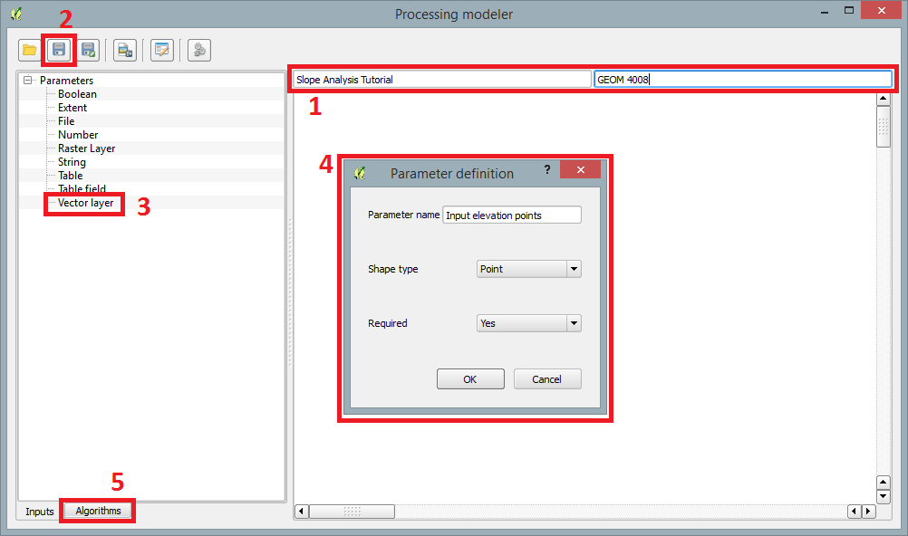
Before creating the model, you must enter a desired model name and group name (1). I named my model "Slope Analysis Turotial" under a group name called "GEOM 4008". Once a model and group name have been enter, select Save (2), and save the model to your desired folder. I would recommend creating a folder just for QGIS models under this project.

To begin your model, you'll first have to add an input parameter. On the left side of the modeler window, select Vector Layer (3). That will then display a Parameter definition (4) window. Enter the Parameter name as Input elevation points (or something similar), Shapefile to Point, and Required to Yes. Select Ok.

Now navigate to the Algorithm (5) tab, to being adding geoprocessing algorithms.

Adding Geoprocessing Algorithms

Inverse Distance Weighted (IDW)

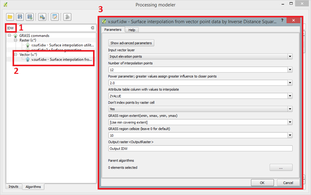
The first algorithm that will be added is an Inverse Distance Weighted (IDW) interpolation. This particular algorithm can be found by doing a search filter for IDW (1), and select v.surf.idw (2) under GRASS Commands.

A window will open asking for interpolation specifications (3). Enter the specifications that you desire.

Make sure that the Input layer is the elevation point data initially added.

For my slope analysis, I had to enter ZVALUE into the Attribute table column with values to interpolate field because the column under the carpdem Attribute Table used for elevation points is named ZVALUE.

I also used a GRASS region cellsize of 10. This can be changed if you'd like, although it may take longer to process with a smaller cell size value. Also add an Output raster name of your choice. Select OK.

Slope

Following the IDW interpolation, a slope map expressed in degrees will be created using the IDW output.

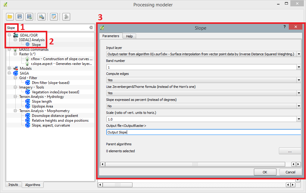
Execute a search filter for Slope (1), and select Slope (2) under GDAL/OGR.

This will display a window for the Slope geoalgorithm (3). Leave the field parameters as default except for Slope expressed as percent to No. Make sure that the Input layer is the initial IDW output created (algorithm 0).

Also add an Output raster name of your choice. Select OK.

Aspect

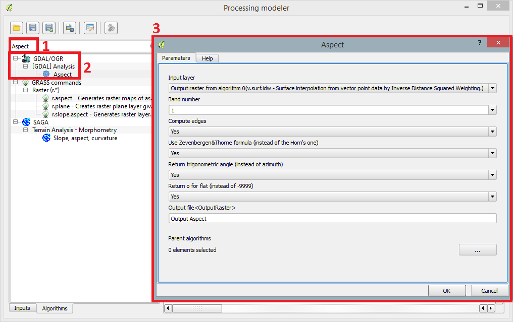
Execute a search filter for Aspect (1), and select Aspect (2) under GDAL/OGR.

This will display a window for the Aspect geoalgorithm (3). Leave the specifications as default. Make sure that the Input layer is the initial IDW output created (algorithm 0).

Also add an Output raster name of your choice. Select OK.

Hillshade

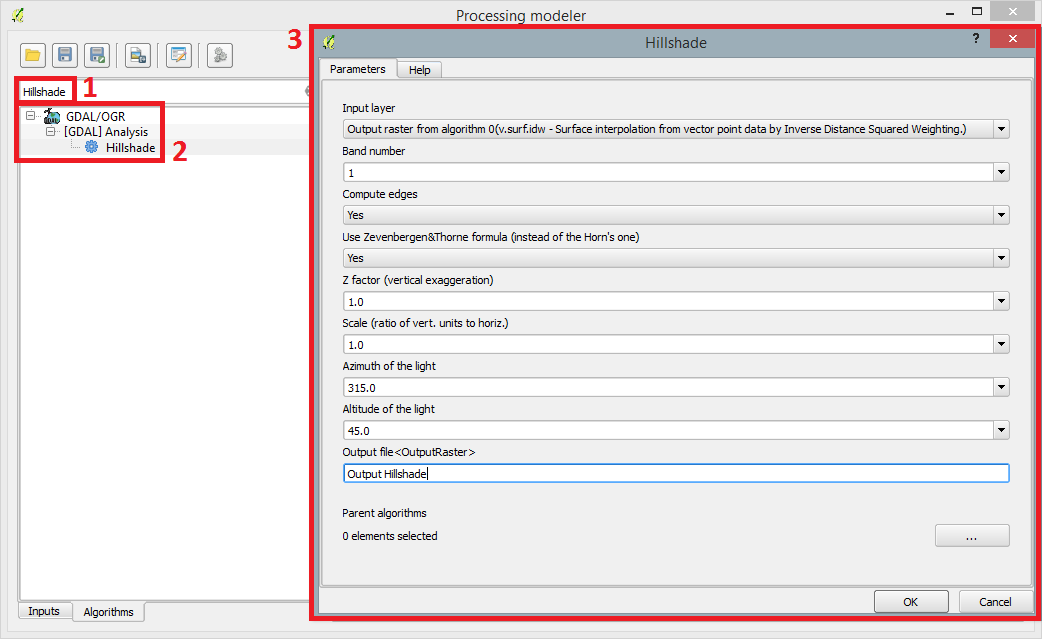
Execute a search filter for Hillshade (1), and select Hillshade (2) under GDAL/OGR.

This will display a window for the Hillshade geoalgorithm (3). Leave the specifications as default. Make sure that the Input layer is the initial IDW output created (algorithm 0).

Also add an Output raster name of your choice. Select OK.

Running a model

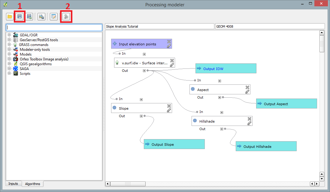
Once all of the geoprocessing algorithms have been added, the model should look similar to capture below.

Make sure that you Save (1) the model before Running the model (2).

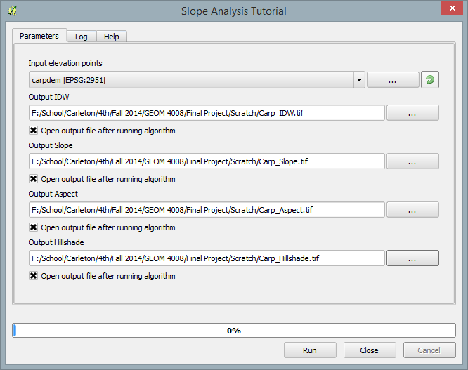
When the Run model button is select, a window the same as the capture below will appear.

In this window make sure you save the output files to an appropriate destination folder. Select OK to run the model.

Once the model is finished running, the output raster layers will be displayed in the Layer toolbox on the left side.

Displaying output rasters from model

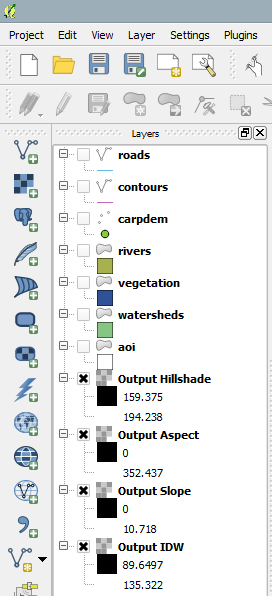
Once the model is run and the output rasters appear in the Layer toolbox. They will only appear as single band image styles.

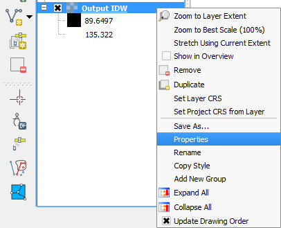
One way to change this is to change this right click on Output IDW, select Properties.

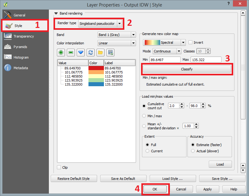
A Layer Properties window will appear. Navigate to Style (1), select the Render type to Singleband pseudocolour (2). Under Generate new colour map settings, the properties can be changed to your personal desire. For my output I selected a Continuous mode and selected Classify (3), then OK (4).

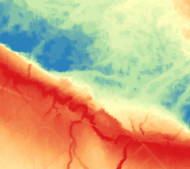
This process can be done for any of the output raster layers. The IDW output was done as an example. The output should look similar to the capture below, depending on the cell size used in the modeling process.

Exporting your model

As a Python script

When your model is finished you can export the model as a Python script.

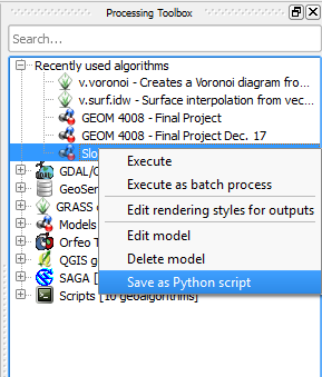
To do so, right click on the model in the Processing toolbox and select Save as Python script.

This Python script can be edited in a program such as Notepad++.

As an image

If you'd like to print out the model or include it in a report. It is possible to save the model as an image for future reference.

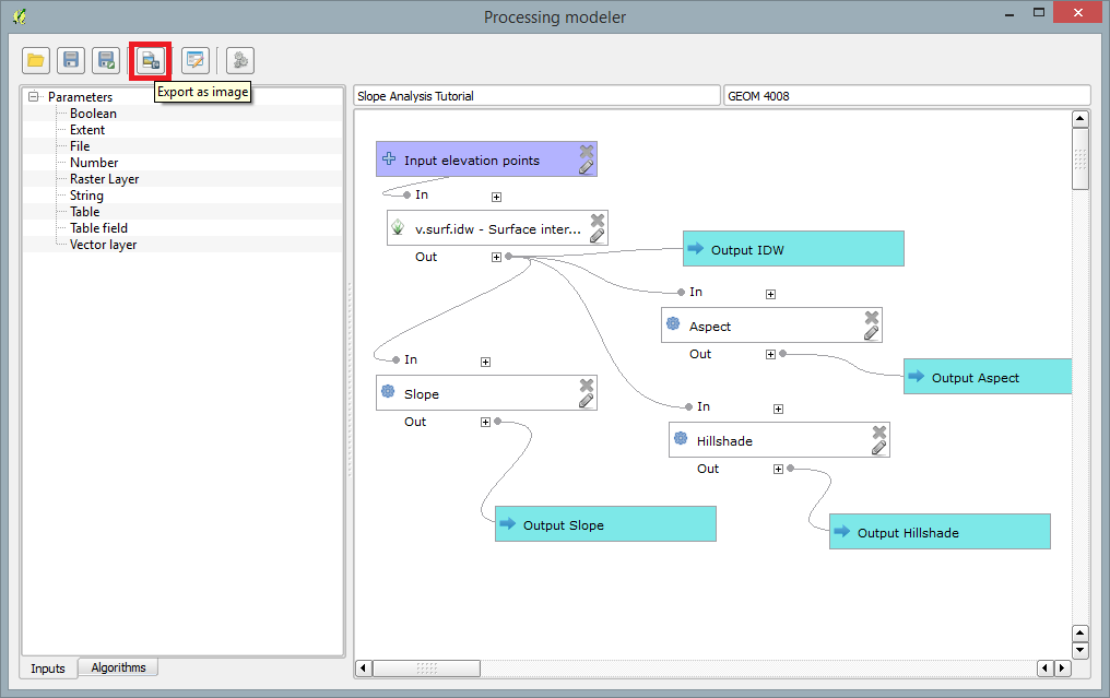
Just re-open your model again from the Processing toolbox and select the Export as image button in the modeler window.