Exploring Hydrological Analyses using ILWIS
Contents
- 1 Purpose
- 2 Introduction to ILWIS and the Project Tutorial
- 3 Methods
- 4 Conclusion
- 5 References
Purpose
This Wiki tutorial has been produced for the purpose of exploring and describing the methods used for hydrological analyses in ILWIS (a FOSS4G program). The objective of this tutorial is to provide users with a better understanding of how the hydrological analyses within ILWIS works, in addition to providing the instructions necessary to reach the desired output for their study region. Additionally, this tutorial will allow for comparison of ILWIS and SAGA GIS, using the same data for analysis as the Exploring Hydrological Analyses using SAGA GIS tutorial from 2013.
Introduction to ILWIS and the Project Tutorial
ILWIS stands for "Integrated Land and Water Information System". It is a open source Geographic Information System software program that was designed to be a user-friendly integrated software that contains both raster and vector processing capabilities, allowing for both analyses on remotely sensed images, vector maps and numerous spatial modeling abilities. ILWIS was developed by the International Institute for Aerospace Survey and Earth Sciences (ITC) in The Netherlands. This tutorial will focus on its ability to use Digital Elevation Models (DEMs)to run hydrological analyses of a study region. More information about this product can be found on the ILWIS Website
This project will focus on hydrological analysis of Okanagan Lake, a popular tourist destination in British Columbia, Canada. The tutorial will cover topics such as Aspect mapping, Slope mapping, Watershed Delineation mapping and Wetness Index mapping through the use of ILWIS hydrological analysis tools.
Methods
Data and Programs
In order to carry out this exercise, a DEM of the area of interest is needed. For this project a open source DEM was obtained using the Geospatial Data Extractiontool created by Natural Resources Canada.
For DEMs located outside of Canada open source DEMs can be obtained from ASTER and SRTM Global Digital Elevation Model - USGS
This turtorial explores the hydrological toolset for ILWIS, but the use of open-source program QGIS is needed as well. This can be downloaded fromthe QGIS website
Getting Started
Before starting any analysis, create your working folder and ensure all data needed for the exercise are in this folder. Keeping all your data in one folder will make analysis easier.
Starting ILWIS
ILWIS 3.08.03 can be downloaded for free from 52 North.The newer version of ILWIS 3.08.04 is available but do not download this one, as a bug does not allow you to import DEMs into this version.
- Ensure that ILWIS 3.08.03 is properly installed on your computer
- Locate ILWIS from the Program list and double click on the icon to launch program.
- ILWIS main page will open
- Use the ILWIS Navigator Tab to locate your working folder. The Navigator lists all drivers and directories.
INSERT main page picture here
Figure ??: Screenshot of ILWIS Interface
Importing DEMs
1) Click Operations --> Import/Export --> GDAL (Geospatial Data Abstraction Library)
printscreen
2) An Import window will open
3) Click to the DEM you want to import and ensure that the import format is Use GDAL.
5) Give your Output DEM a name and click OK
6) To view your DEM go to Operations -> Visualization -> Show map. A new window will open with the DEM.
Projecting a DEM in QGIS
Fill Sinks in a DEM
Creating Buffer
Parts of the criteria set for sitting the landfill are proximities to major roads and water-bodies; therefore buffers are to be created around major roads and water-bodies. To create buffer in ILWIS, follow the steps below:
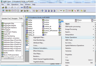
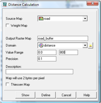
1) Right click on the raster data and scroll to Raster Operations, then choose Distance Calculation
2) Give name to Output Raster Map
3) Choose distance as Domain
4) Specify distance and click show to view the map
5) Repeat the steps 1-4 for other data to be buffered.
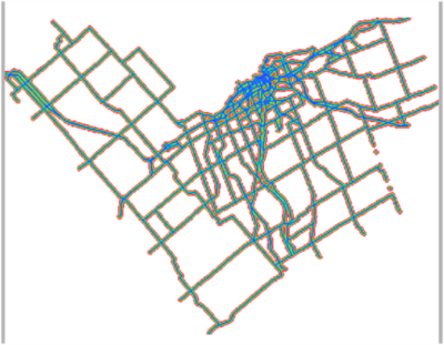
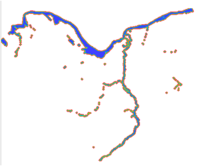
Figures below are the results of the buffer generated:
Figure 9: Screenshot showing Road Buffer
Figure 10: Screenshot showing Waterbody Buffer
Contour to DEM
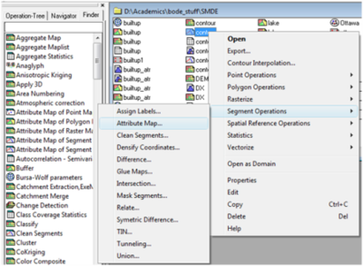
1) Right click on the contour data, Scroll to Segment Operations, then Attribute Map
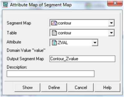
2) Change Attribute to the field that contain the Z values, then give name to Output Segment Map
3) Click show to view the map
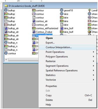
4) Right click on the newly created contour data (Contour_Zvalue) and scroll to Contour Interpolation
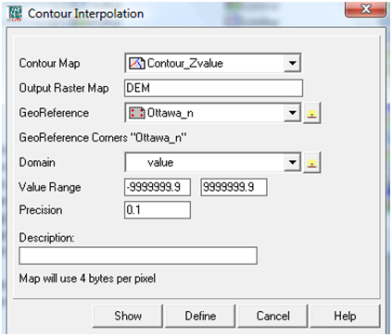
5) Give Output name (DEM), choose the GeoReference created earlier, leave Domain as value
6) Click show to view the map
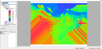
Figure 11: Screenshot showing DEM
DEM to Slope
Creating DFDX and DFDY
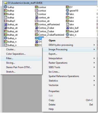
1) Right click on DEM data, choose Image Processing>Filter
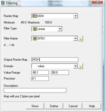
2) Choose Linear as Filter Type and Filter name to DFDX
3) Give Output name and click show to view the map
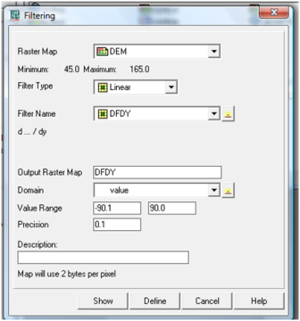
4) Repeat the same process to create DFDY
Creating Slope
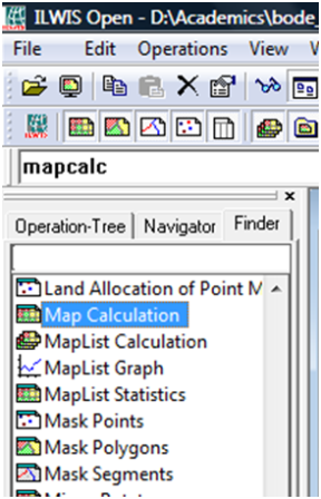
1) From the Finder Table of Content, double click Map Calculation
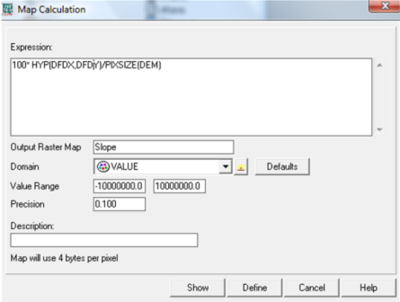
2) Type this formula: 100*HYP (DX, DY)/PIXSIZE (DEM) into the Expression Space
Note: Change DX, DY and DEM using your own data
3) Give Output name and choose value as Domain
4) Click Show to view the map
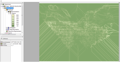
Figure 12: Screenshot showing Derived Slope
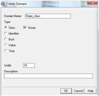
Creating Domain for Slope Classification
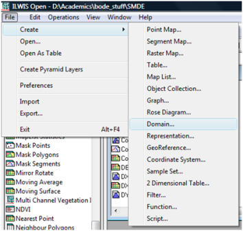
1) Click File, then Create and click on Domain
2) Give Domain Name, Check Class and Group
3) Click Ok to Continue
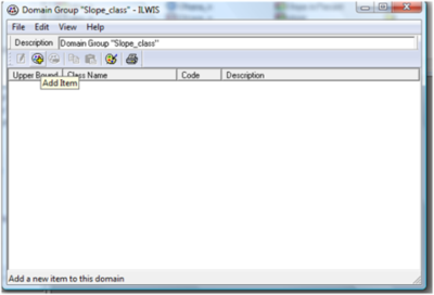
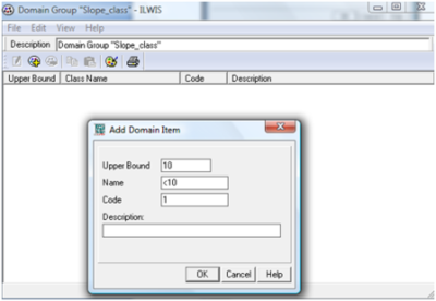
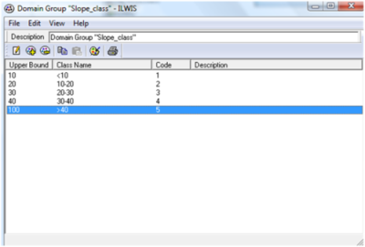
4) Click on add Item to add all classes
Combining Slope with Domain
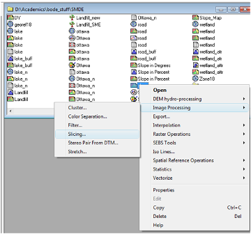
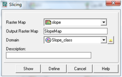
1) Right click on the Slope data, Go to Image Processing and Click on Slicing
2) Give Output Name and Choose Domain created earlier as Domain (Slope_class)
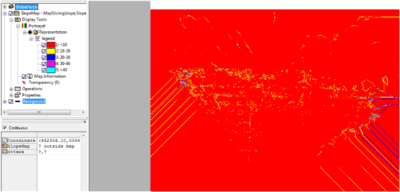
3) Click Show to view the Slope Classification Map
Figure 13: Screenshot showing Slope Classification
Spatial Multi-Criteria Evaluation Analysis
Getting Started with SMCE
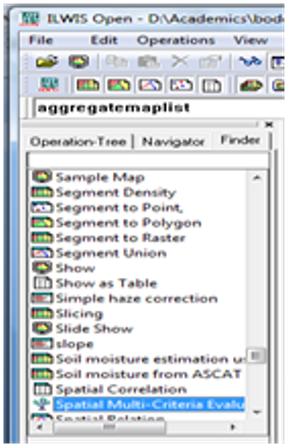
1) From the Operation Tree, double click on Spatial Multi-Criteria Evaluation
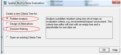
2) Both the Problem Analysis and Decision Making modules will be used to find the suitable Landfill sites
3) Select on Problem Analysis and click OK to open the SMCE workspace
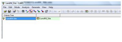
4) Click File>Save to save the SMCE project
5) Double click on New Goal to rename it and click on ‘filename given’ to give output name
Adding factors and constraints data
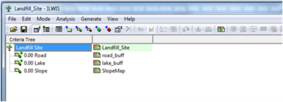
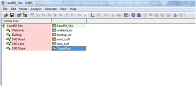
1) Click on insert Spatial Factor icon or click Edit>Insert>Spatial Factor to inset all 'Factors' data
2) Click on Insert Spatial Constraint icon or click Edit>Insert>Spatial Constraint to insert all 'Constraints' data
Standardize factors and constraints
1) To standardize factors, change to Multi Criteria Analysis Mode
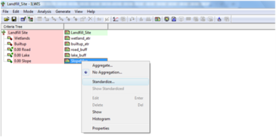
2) Right click on the factor data and choose standardize
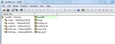
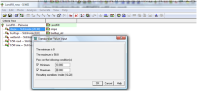
3) To create standard for slope, enter the minimum and maximum suitable slope values
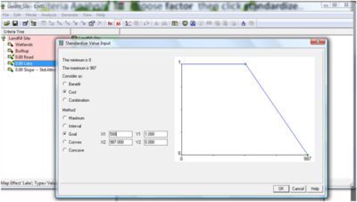
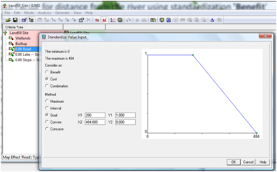
4) To standardize the road data, right click on the road raster data and choose standardize.
5) Here, I chose Cost and Goal as Method and entered range scores
6) Repeat the same steps to standardize waterbody
Assigning weight (Pairwise)
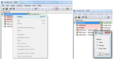
1) To assign weight, right click on the goal name (Landfill) under ‘Criteria Tree’ and choose Weigh or click on Weigh icon.
2) I chose the Interactive ‘Pairwise Method’ and clicked Ok to continue
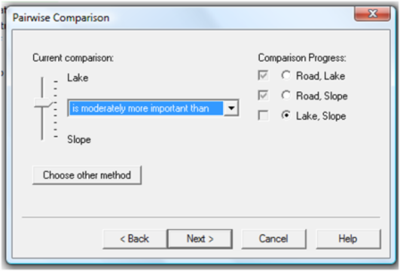
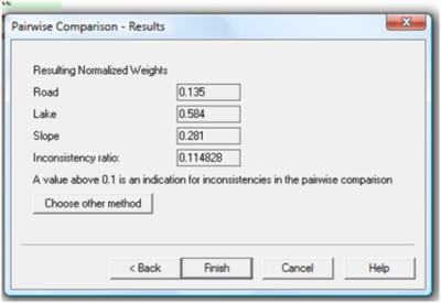
Below are the weights assigned to each factor:
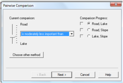
3) Here, I clicked the drop down box and I chose ‘Road is moderately less important than Lake
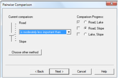
4) Repeat the same for Road, Slope and Lake, Slope
Note: There are other two methods of assigning weights which also be used
Pairwise Comparison Results
Running Spatial Multi Criteria Evaluation Module
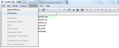
1) To run the SMCE module to create the suitability map for Landfill, click on Generate and choose ‘All Output’
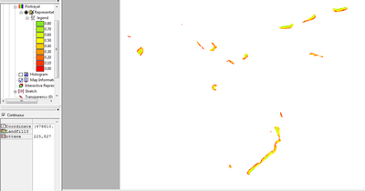
2) Wait a while for the analysis to finish and click Ok to view the map
Figure 14: Screenshot showing Suitable Landfill Sites
Interpretation of Result
SMCE map shows values ranging from 0-1; a value of 0 denoted with colour Red indicates less suitable areas. The more the values move towards 1, the more acceptable such areas are, i.e. transitions from Yellow to lemon and finally Green indicates the most suitable sites.
Conclusion
This tutorial showed the steps required for suitability mapping for landfill in the City of Ottawa, using the analytical functions of SMCE module in ILWIS software. Decision Tree wizard was used to add factors and constraints; to standardize and assign weights to the constraints and factors for successful execution of the decision processes. Finally, SMCE analysis was carried out to derive the suitability map for the landfill.
References
- Agus (2011), Modeling Spatial Analysis for Identifying Landslides Areas in Sumedang
http://www.scribd.com/doc/76923076/Analysis-spatial-using-ILWIS
- Mohammed A. Sharifi and Vasilios Retsios,(2004), Site selection for waste disposal through spatial multiple criteria decision analysis
http://www.itl.waw.pl/czasopisma/JTIT/2004/3/28.pdf
- Multi Hazard Risk Assessment
http://www.ecapra.org/sites/default/files/documents/Book%20Multi%20Hazard%20Risk%20Assessment_0.pdf
- 52 North
