Exploring Standard Statistics in QGIS

Purpose

The purpose of this Wiki tutorial is to present the user with further information on the basic spatial statistic tools available within QGIS. Step by step instruction will demonstrate how each tool can be used to perform statistical analysis on vector datasets. Furthermore, this tutorial will not cover detailed explanations on how to use project specific statistical tools (i.e. hydrological and terrain tools) as there are tutorials focused specifically on those toolsets that can be found on the main Wiki page. Instead there will be descriptions of these standard statistical tools and discussion on what they are typically used for. This tutorial will also touch on the limitations of such tools in QGIS and how the integration of other open source software can reduce these limitations.

Introduction

Geospatial analysis composes the root of all geosciences. Spatial statistics were uniquely created to analyze vector data in order to find patterns and relationships within a distribution which is what makes GIS software such a powerful tool. Standard spatial statistic tools that are available within QGIS include basic statistics, nearest neighbour analysis and mean coordinates which will be the main focus in the following tutorial. These standard tools are advantageous to any user who is attempting to further understand a vector dataset apart from the initial visual representation. Although simple, standard statistics tools are arguably the most valuable when analyzing a new dataset. QGIS is a very powerful free open source software (FOSS) but it still has its limitations. Integration of a second FOSS, GRASSGIS, can introduce ways of dealing with more complex statistical problems and close the gap on some limitations within QGIS.

Materials

About QGIS

Quantum GIS, better known and QGIS, is arguably the most powerful and commonly used free open source geographic information system software available. It allows the user to create, edit, visually represent, analyze and publish information. It is available for download on a variety of operating systems from Windows, Mac, Linux and BSD with recent efforts working towards compatibility with Android. QGIS is licensed under the Creative Commons Attribution-ShareAlike 3.0 license (CC BY-SA).

Download QGIS

The most recent version of QGIS is 2.12.1 Lyon which was released on November 27, 2015. It is available for download on their Official Website. Download and install the current version of QGIS for your operating system in order to follow along with the following step-by-step tutorial.

Data Acquisition

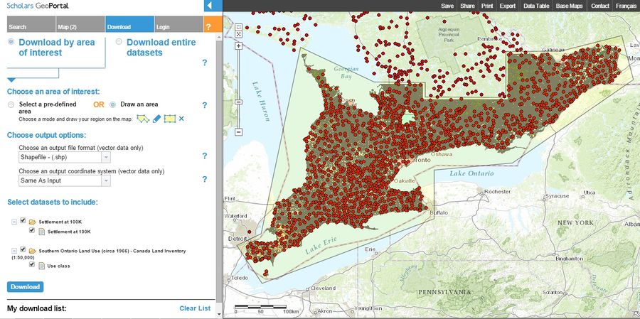
There are numerous resources available to acquire spatial data for use within GIS software such as the Ottawa Open Data Catalogue and Scholars GeoPortal. For the purposes of this tutorial, we will be using data taken from the Scholars GeoPortal which is accessible online using your Carleton University student login through the MacOdrum Library website. The data required for this tutorial is the Ontario population data file entitled Settlement at 100k and the Ontario land use data entitled Southern Ontario Land Use (Circa 1966) – Canada Land Inventory (1:50,000).

Settlement at 100k: This is a point dataset marking locations of populated areas across the province of Ontario, Canada. Southern Ontario Land Use (Circa 1966) – Canada Land Inventory (1:50,000): This data set details the land use planning initiative set out by the Ministry of natural resources (MNR) that have been established for large geographic areas across Southern Ontario, Canada.

Click the following link and enter your Carleton University student login to access the Scholars GeoPortal database.

1. Under the Search tab, search and add the two datasets to your working map.
2. Under the Download tab, select the Download by area of interest option then select Draw an area and choose the polygon shape as your mode of drawing. Manually select the area you want to download data for by drawing directly on the map. Double click to end your selection.
   1. 

      Figure 1: Image of Scholars GeoPortal showing map selection of datasets ready for download.
3. Click the download button in the bottom left hand corner of your screen. Below this button is your download list and is the location where your files will download to.
4. Once the files have completed downloading to your download list, click on each item to download them to your desktop. Note that these files are large and will need to be unzipped before being saved to your preferred location.

Tools and Methods

Getting Started

Before any analysis can be done, your project projection must first be set and then the datasets being used must be imported into QGIS.

Setting Project Projections

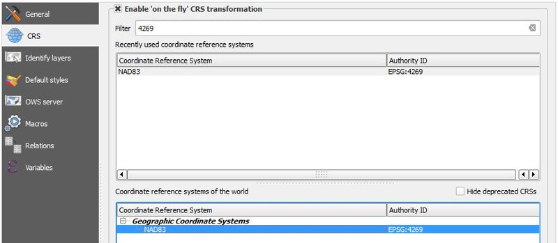
There should not be a need to project the layers as they should both already share the same projection, NAD83. However, it is necessary that your project be set to share the same projection as your data layers.

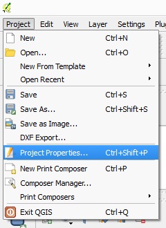
1. To set your project projection, open Project Properties under the Project tab.
   1. 

      Figure 2: Project tab menu.
2. Choose the appropriate projection for your project, click OK.
   1. 

      Figure 3: Project properties window showing project projection selection.
      For more information on re-projecting data layers, click | here.

Importing Data

To import data, click the Add Vector Layer button,

Select the desired dataset.

Playing with Symbology

Once your data layers have been added to your working project, take time to play with the symbology and express the data in a visual way that suits your needs. In this tutorial, the Land Use dataset was expressed in a more simplistic way by grouping similar land classes together and using a more appropriate colour scheme. For additional information on using symbology in QGIS, click | here.

---

Basic Statistics

Basic statistics are a set of values calculated from a dataset known as, the mean, the mode, the median and standard deviation and are exactly what their name suggests, the most basic statistics. They form the basis of statistics and are some of the most valuable to calculate. Often used as tools for the organization on larger datasets.

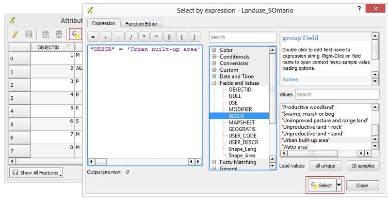
Using the Land Use dataset, one might want to know the area of land in Southern Ontario that is classified as a particular land use. For example, the area of land considered to be built up urban area.

1. To do this, query to select all polygons from the data layer that are classified as build up urban area. This is done in the data layers attribute table.
   1. 

      Figure 4: The Select by expression window in the attribute table used to query for desired attribute in a data layer.
      For more information on querying in QGIS, click | here.
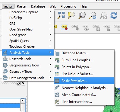
2. Once your selection is complete, open the Basic Statistics window under the Vector > Analysis Tools tab.
   1. 

      Figure 5: Vector > Analysis Tools tab menu.
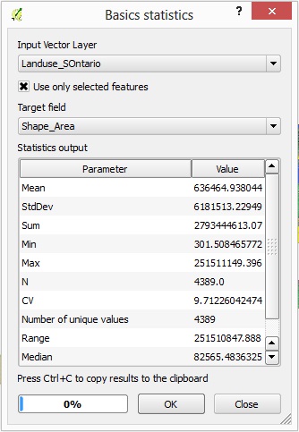
3. In the Basic Statistics window, select your layer of interest. Be sure to check the box ‘Use only selected features’. The target field should be the field that the statistics are being calculated for, in the case of this tutorial, Area. Click OK.
   1. 

      Figure 6: Basic Statistics Window showing statistics for area of urban land use in Southern Ontario.

Results will be shown in the units that correspond to your project projection. In the case of this tutorial, area statistics are displayed in m2, where total area is the sum at 2.79E109m2.

---

Nearest Neighbour Analysis

Nearest neighbour analysis, similar to the Distance Matrix tool, is a tool that calculates the mean distance of all point files in a data layer to the next nearest point. Output results of this tool include; Observed Mean Distance, Expected Mean Distance, Nearest Neighbour Index, N and Z-Score. These values are typically used in distribution modeling and cluster analysis.

In this tutorial we want to know the mean distance that is observed between all population settlements to try and understand their distribution in Southern Ontario.

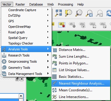
1. Open the Nearest Neighbour Analysis window under the Vector > Analysis Tools tab.
   1. 

      Figure 7: Nearest neighbour tool under the analysis tools menu.
2. Select the appropriate input vector layer, click OK.
   1. 

      Figure 8: Nearest neighbour analysis window showing results in degree units.

Results of this analysis are valuable, however, under the current projection the output distance is given in degrees. If meter units are desired, the data layers would have to be re-projected to a different map projection before nearest neighbour analysis is performed.

---

Mean Coordinates

Mean coordinates is an analysis that identifies the mean, or average, location of specific points in space or a geographic centre. It tool creates a new point file as a means of representing the output location.

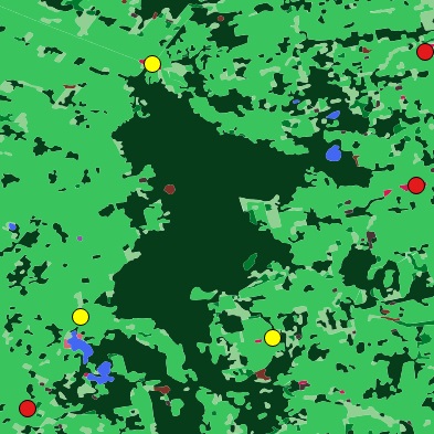
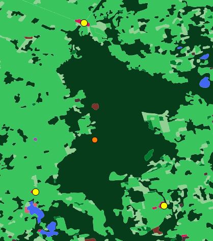
A basic use of this tool could be as simple as determining an area located equally between three known populations to create new cropland.

1. Select the point locations that you wish to find the mean coordinates of. This can be done via query in the attribute table as we previously done in section 4.1, or the locations can be manually selected using the Select features by area or single click tool on the Attributes Toolbar. For multiple feature selection, select while simultaneously holding the Ctrl button on your keyboard.
   1. 

      Figure 9: Attributes Toolbar with red box highlighting the Select features by area of single click tool.
   2. 

      Figure 10: Image clip of the working map. Yellow circles indicating manually selected population locations.
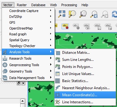
2. Open the Mean Coordinates window under the Vector > Analysis Tools tab.
   1. 

      Figure 11: Mean Coordinate tool under the Analysis Tools menu.
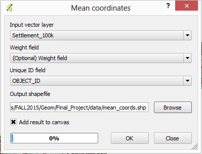
3. Select the appropriate input layers and create an output layer name, click OK.
   1. 

      Figure 12: Mean Coordinate window.
   2. 

      Figure 13: Map clip of resulting output point file (in orange) marking the mean coordinate and new crop location.
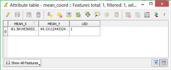
4. The resulting output shapefile represents the mean coordinate point of the three locations. This is the location that the new crops will be made. X and Y coordinates of this centre point can be down in the point files attribute table.
   1. 

      Figure 14: Table showing spatial coordinates for the mean coordinate output.

Integration with GRASS

About GRASS

The most recent version of QGIS is 2.12.1 Lyon was released on November 27, 2015 and is available with integration of GRASS version 6.4.3. (ADD MORE…)