Thematic Mapping using GrassGIS

Purpose

The purpose of this tutorial will be to use multiple tools in Grass GIS that will manipulate vector data. The example to be used in the tutorial will be the analysis of Ottawa City neighbourhoods to determine where would be the most appropriate place to live as a student attending Carleton University. This tutorial will use the following tools:

Extract- selection by attributes, Patch- patch vector layers together, Select- selection by location,

Overlay- clip tool, and Buffer- generate buffer

There will also be some coding using the command console for tools that are not included in the WxGUI.

This is a basic introduction to thematic mapping using the Grass GIS software vector analysis capabilities.

Introduction

The purpose of this tutorial is to show how to represent and visually understand spatial vector data using thematic mapping. This tutorial addresses a problem that many individuals have when looking for new housing. The issue is of finding the most appropriate area to live in based on a multitude of factors. This tutorial focuses on Carleton University students in particular and the confusion or misinformation in choosing an appropriate place to live in Ottawa off campus. This issue is addressed through the use of thematic mapping and criteria outlined by the Carleton University Off-Campus Housing Office. For the sake of time there are only three main factors looked at when looking for where to live, they are: Rent price, Crime/safety, and Proximity to the university.

This tutorial will show how to add and manipulate relevant spatial data in order to make thematic maps representing the criteria students are looking for. The tutorial can act as a precursor to a tool that can be implemented by Carleton University to develop a thematic map that students without the GIS knowledge to use. There is a lot of potential for this to be used for more than just students as well since it helps people find places to look for housing based on ideal criteria.

The data used for this tutorial are available on the Carleton University library website as well as through the City of Ottawa, Ottawa Neighbourhood Study, OCTranso, and Ottawa Police websites.

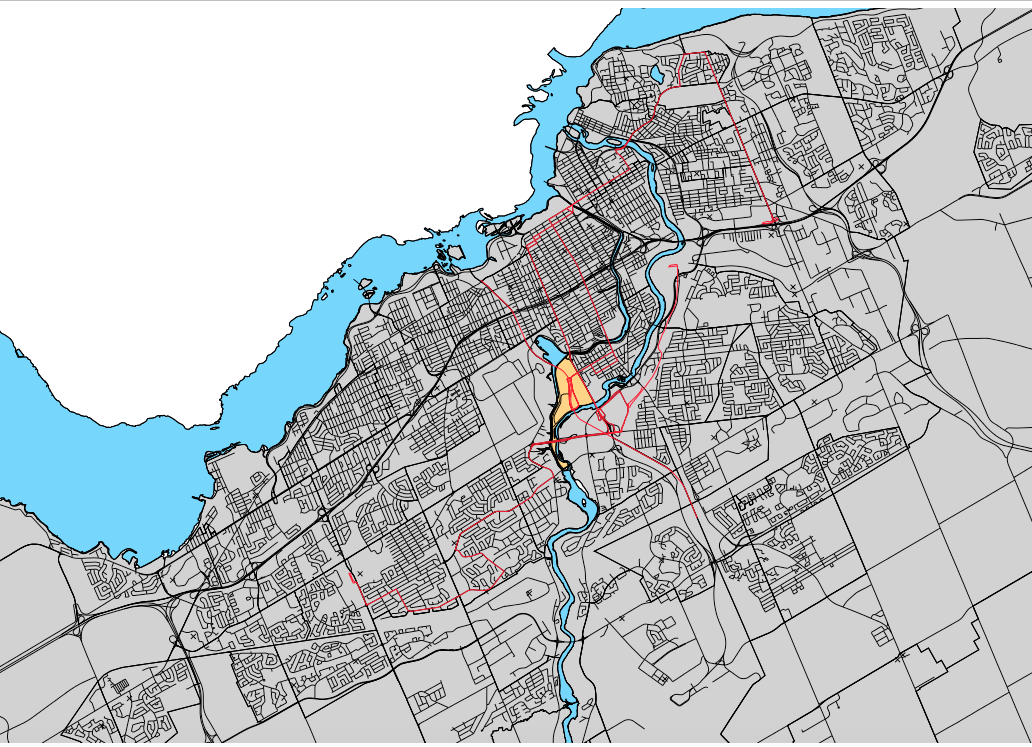
Figure 1: The study area of the tutorial central to Carleton University.

Software

Grass GIS

This software is open source and can be downloaded at the Grass GIS download page.

Grass GIS operates on Mac OS and Linux properly, if using Microsoft it is recommended to use a Linux virtual machine.

If you choose to run Grass GIS on Mac OS and are currently operating Mac OS X 10.11 (El Capitan) and above you will need to restart your computer in recovery mode. This does not do any hard to your computer and allows you to easily run Grass GIS on the newer Mac operating systems. (Note: You can download the Grass frameworks and software before restarting in recovery mode)

To do this simply follow the instructions below:

1. Restart your computer and as soon as the screen turns black hold down Command + R on the keyboard until the Apple logo appears on your screen.

2. Open the Utilities menu and click Terminal

3. When the Terminal Window opens type in: "csrutil disable" and then press Enter

4. Restart your computer again

5. You should now be able to run Grass GIS

Data

Data Identification

The data to be used in the tutorial was determined through the identification of criteria and research into the availability of the data required. Carleton University library had all of the data compiled from their original sources. The data available is relatively recent in terms of the last studies conducted (Census) and explains the criteria we are looking for. The data sets included are as follows:

1. Ottawa Thematic Data

2. Ottawa Police Crime Statistics

3. OC Trasnpo 2015 Route Data

4. Ottawa Neighbourhood Study (Both shape files and statistical data)

Data Links and Explanations

1. Ottawa Thematic Data

This data package includes most of the thematic data in Ottawa such as city boundaries, roads, rivers, and parks for example. The shapefiles used from this dataset in this tutorial are Roads, Rivers, Railways, Parkland, Police/Fire/Ambulance, and Hospitals. This will let us how areas of the city important to people looking for housing such as distance to hospitals.

2. Ottawa Police Service

This data package includes crime statistics by Ottawa City Ward. The file we are interested for this tutorial is the 2015 shapefile since it is the most recent compilation of Ottawa crime. The file will allow us to determine the average total crime and solving rate in order to rate safety on areas based on crimes committed.

3. OC Transpo Transit Routes

This data package includes the bus routes around Ottawa. The shapefile of interest it the 2015 Transit routes since it is the most recent addition to the file. This will allow is to determine which bus routes are important to the project.

4. Ottawa Neighbourhood Study

This data packages divides the City of Ottawa into the different neighbourhoods that will be used as the locations for potential residency. This is because the financial information for these different neighbourhoods is readily available to be added to the shapefile.

*Data packages are available on the Carleton University Library website to Carleton students or alumni.

**Files are zipped, an unzipping tool is recommended.

Tutorial

Download Data

Download the data from the provided links in the Data section.

Note: for instructions on how the TransitRoutes_2015 data should be imported, please see step 5.5 Importing the Bus Routes that Service Carleton University.

Setting up Grass GIS Directory and Location

The following steps help explain how to choose a Grass GIS, location, and set projection.

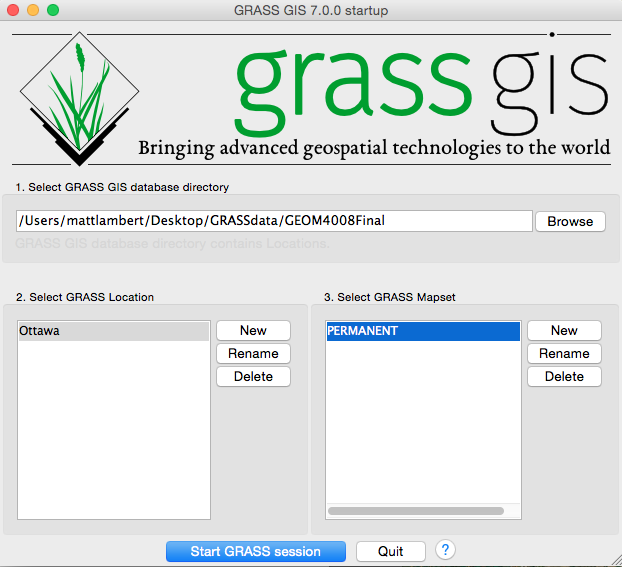
1. Create a new file and connect to it through the browse option to make it your directory. Create another file in your directory and name it something relevant to the project, this will become the location folder. Place all of the data into the location folder so we can draw upon it later. Use PERMANENT as the default mapset.

Figure 2: Grass GIS start page where you select directory and location.

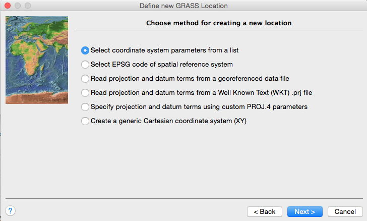
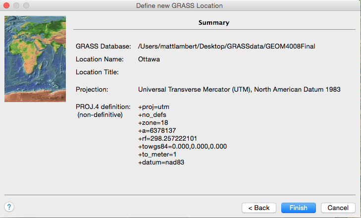
2. Set the projection for your newly created location folder to UTM zone 18, and the NAD 83 datum set for this project since that covers the City of Ottawa.

Figure 3: (Top) choose the set projections from a list. (Bottom) a picture of chosen projections.

Adding Layers to Project

The following images help explain how to add the vector layer data that will be used in the tutorial.

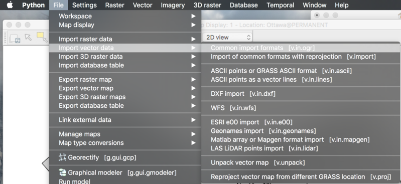
1. Click on the file tab and scroll down to Import vector data, then choose Common imports format [r.in.gdal] as seen in Figure 4.

Figure 4: How to get to the import vector data tool in Grass GIS.

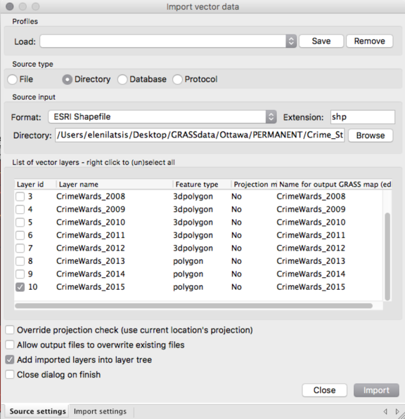
2. Choose the Directory option under source input. Source input choose ESRI Shapefile and search for the CrimeWards_SHP layer folder in the directory. Next choose the CrimeWards_2015 as seen in Figure 5.

Figure 5: How to select layers to import into Grass GIS.

Isolating the Study Area (Carleton)

This section will show how to isolate Carleton University into its own layer since it will be called upon in later steps.

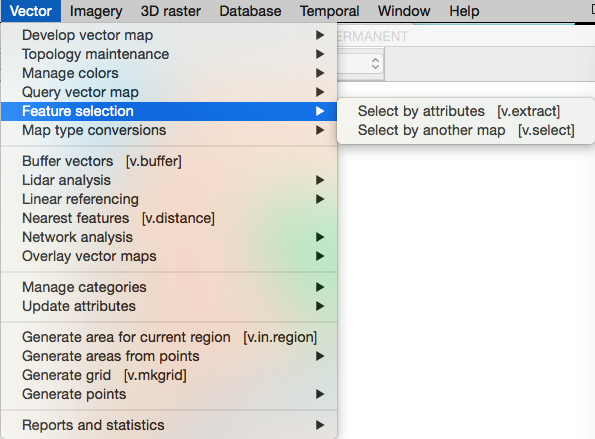
1.To isolate Carleton we will use the Select by attributes tool or v.extract command this can be found in the vector tab as shown in Figure 6.

Figure 6: How to access the Selection by attributes tool in the Grass GIS GUI.

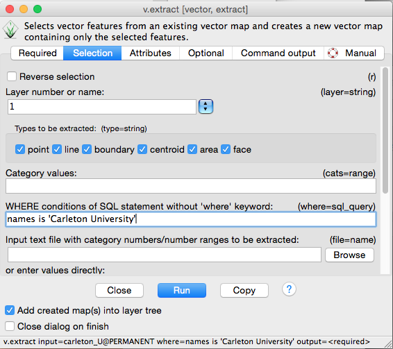
2. Once in the Select by attributes window select the ONSNeighborhoods2012_SmallFile layer as the vector map, then select the tab that says Selection and type in the SQL command name is 'Carleton University' . This will select the Carleton University neighbourhood and extract it into a separate layer to be used later. This step can be seen in Figure 7.

Figure 7: How to write the SQL statement required to extract Carleton University into a separate layer.

Importing the Bus Routes that Service Carleton University

For this step, we need to import the bus routes that stop through Carleton University's campus: OTrain, #7, #4, and #111.

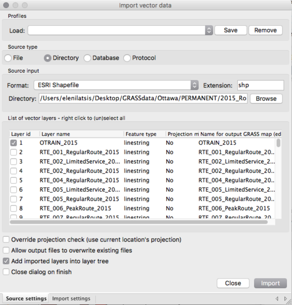
These can we found in the TransitRoutes_2015 file and should be imported as four seperate layers.

Figure 8: Importing the bus routes that service Carleton University

Merging the transit routes into one layer

This step will merge the bus routes into one layer, this will be beneficial in saving time when querying the transit routes in later steps.

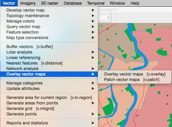
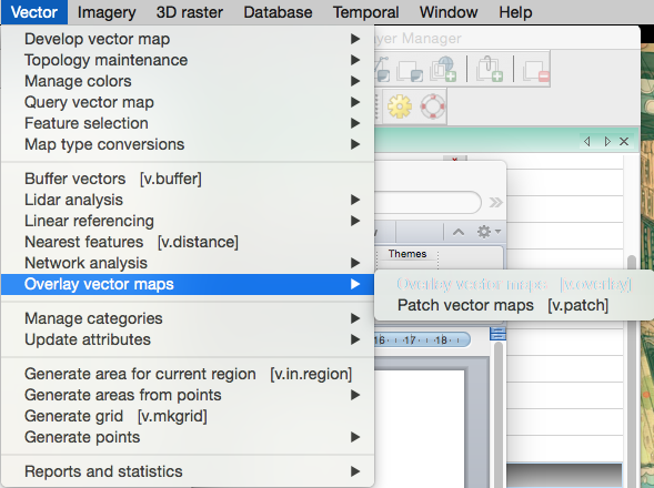
1. To merge the different transit routes into one layer we will use the Patch tool. This can be found in the vector tab as shown in Figure 9.

Figure 9: How to select the Patch tool in the Grass GUI.

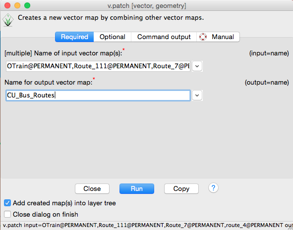
2. Once in the Patch window, select the transit layers imported in the previous step as the input vector maps as seen in Figure 10. Name the output vector map CU_Bus_Routes.

Figure 10: Shows how to operate the Patch tool.

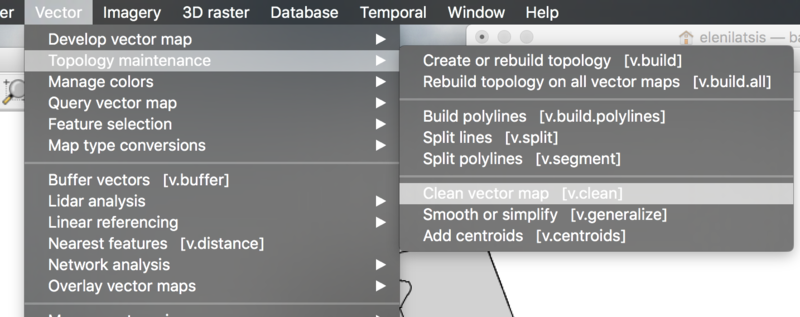
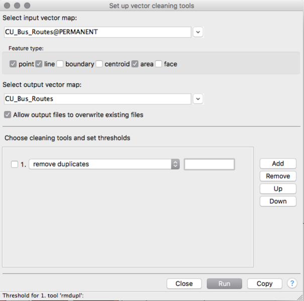
3. It is recommended that you use the Clean vector map tool in order to remove any unwanted duplicates within the merged layer. Please refer to Figure 11 and Figure 12.

Figure 11: How to select the Clean vector map tool in the Grass GUI.

4. Once in the Clean vector map window, select the merged transit layer CU_Bus_Routes created in the previous step, followed by remove duplicates and your desired threshold under the cleaning tools and thresholds section.

Figure 12: How to operate the Clean vector map tool.

Selection of Neighbourhoods Serviced by Transit that Connects to Carleton University

This step will isolate the neighbourhoods that are directly serviced by transit that connects directly to Carleton University. This will be the main focus on choosing where to live since taking more than one bus or train can be a hassle and undesirable.

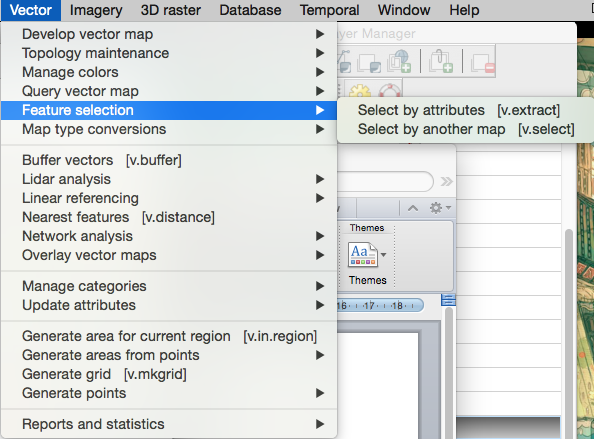
1. Click in the vector tab in the Grass GUI and scroll down to Feature selectionand choose the tool labeled Select by another map or v.select. This tool will query two vector maps together to produce a layer based on the criteria chosen. Figure 13 shows how to get to this tool.

Figure 13: How to navigate the Grass GUI to get to Select by another map tool.

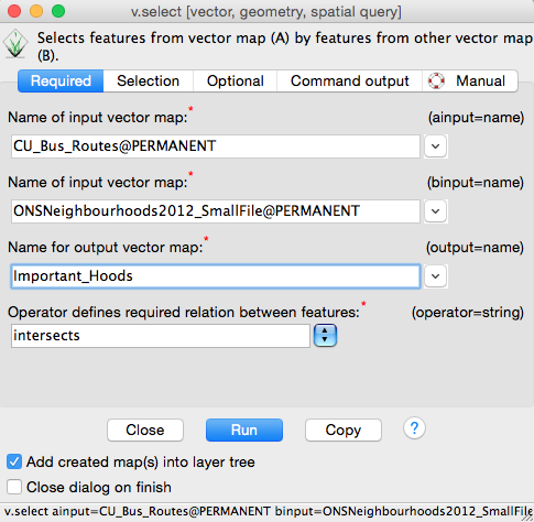
2. Once in the Select by another map window, input the information shown in Figure 14 into the different options. The intersects operator will select neighbourhoods that intersect with the transit routes that connect to Carleton University.

Figure 14: Inputs needed in the selection tool needed to extract the neighbourhoods 'attached' to Carleton University via transit.

Overlay the Crime Wards Layer by the Important Neighbourhoods Layer

This step will overlay the information contained in the crime_wards layer into the newly created important neighbourhoods layer from the previous step. The reason why this is necessary is because the project is using Ottawa's neighbourhoods instead of Ottawa's wards as places to live and the crime data is only available by ward. This will overlay the wards into the different neighbourhoods being looked at.

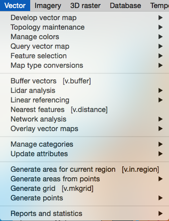
1. Click on the vector tab and scroll down to Overlay vector maps in the Grass GUI and select the Overlay vector maps tool as seen in Figure 14.

Figure 14: Shows the path to get to the overlay tool in the Grass GIS GUI.

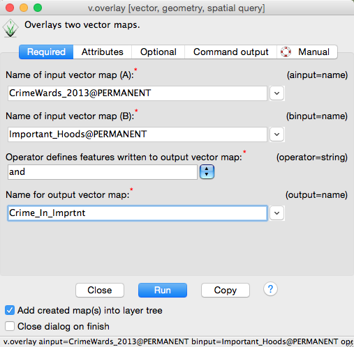
2. Input the information seen in Figure 15 into the Overlay window and choose the and operator. This operator will only choose areas that overlap (i.e where layer 1 AND layer 2 meet).

Figure 15. Shows the input information for the overlay tool.

Creating a Choropleth Map for Crime

This step will create a thematic choropleth map using the total number of crimes committed in each neighbourhood. This will be shown in a colour range from red (Lowest) - orange (Middle) - Brown (High) and all the colours in between those three main colours. This step will use the Grass GIS command console as well as the Grass GUI.

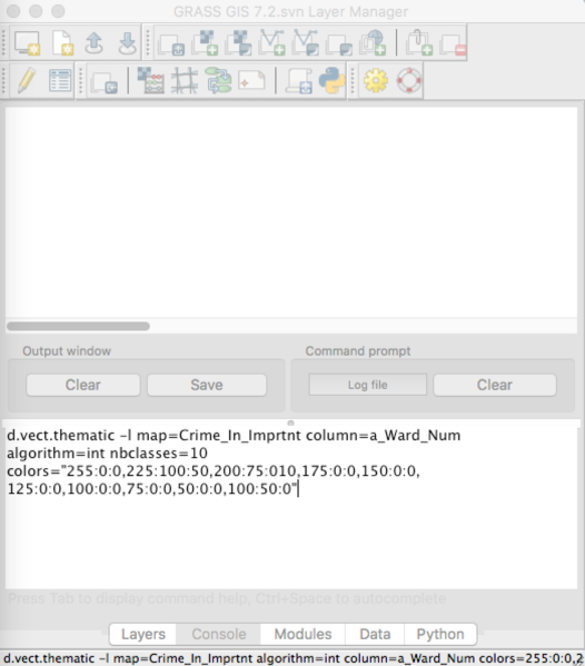
1. On the Layer Manager window, click the Command Console tab and type in the following code in order to create the choropleth map.

d.vect.thematic -l map=Crime_In_Imprtnt column=a_Ward_Num algorithm=int nbclasses=10 colors="255:0:0,225:100:50,200:75:010,175:0:0,150:0:0, 125:0:0,100:0:0,75:0:0,50:0:0,100:50:0"

This can also be seen in Figure 16 below.

Figure 16: How to create a choropleth map in the Grass GIS Command Console.

Note: There is an explanation of all the elements put into the d.vect.thematic command on the Grass GIS help website for further understanding.

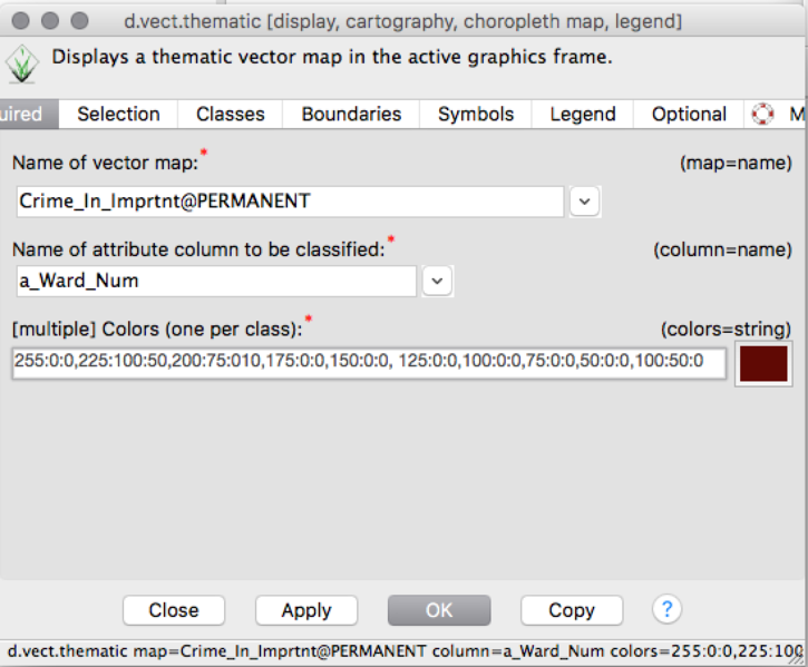
2. Alternatively, you can use the Grass GUI to create a thematic choropleth map, by selecting Add thematic (choropleth) vector map layer. In the window, specify the name of the vector map you want to create, the attribute column you will be classifying (a_Ward_Num), the colours you would like to use, as well as the number of classes. This is demonstrated below in Figure 17.

Figure 17: How to create a thematic choropleth map using the Grass GUI.

Placing Buffers Around Carleton University and the Transit Routes

This step will create buffers around Carleton University and the selected transit routes in order to simulate ideally how close to Carleton University students would live and walk to school and ideally how far away from one of the transit routes students would live away. This project uses 1 km as the ideal distance students would walk to school from home, and 500 m as the ideal distance to live away from a transit route that connects to Carleton University.

1. Click the Vector tab and scroll down to the Buffer Vectors tool or v.buffer command as seen in Figure 18.

Figure 18: Shows how to get to the Buffer tool in the Grass GIS GUI.

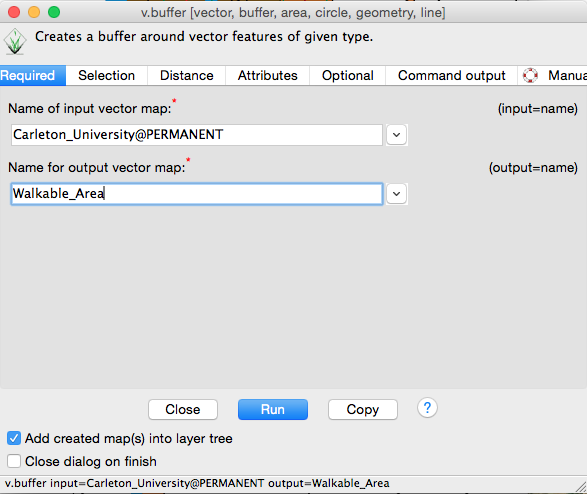
2. select the vector map to put the buffer around and name it something relevant to the project. This can be seen in Figure 19.

Figure 19: Shows how to select the vector map and name the output vector map.

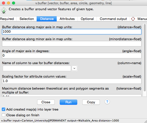
3. Click on the Distance tab and input the distance of 1000 m (1 km) (the map units are in meters since we are projected in UMT coordinates). This will place a 1 km buffer around Carleton University as seen in Figure 20. Once the layer is created make the layer fill transparent so we can see only the outline. This can be done by right clicking the layer in the Layer Manager and clicking on properties/colours then clicking the box that says transparent beside the layer fill colour.

Figure 20: Shows where to input the distance information for the buffer.

4. Repeat the same process but for the bus routes that were extracted in step 6 and use a distance of 500 m.

Extract the Experimental Farm

This step will extract the Experimental Farm neighbourhood that will be used in the next step. This process is exactly like step 4 except using the neighbourhood name of Civic Hospital - Central Park instead of Carleton University since we are interested in that area.

1. Follow and repeat step 4 using the different neighbourhood name.

Overlay the Experimental Farm Layer and the 1 km Buffer Layer

This step will isolate the portion of the Experimental Farm and the 1 km ideal walking distance buffer around Carleton University that overlap. This is to create a blocked out area that shows that there is no actual housing there and is a portion of a large park. This step is exactly like step 8 using different layers.

1. Follow and repeat step 8 using the two different layers. Change the layer fill colour to black once it is created by right clicking it in the Layer Manager window and clicking properties/colour and the layer fill colour box.

Adding a New Column and Data in the Important Neighbourhoods Attribute Table

This step will show you how to add data to the attribute table of a vector map. This project will use the Important neighbourhoods vector map created in step 7 to add average rent prices per neighbourhood.

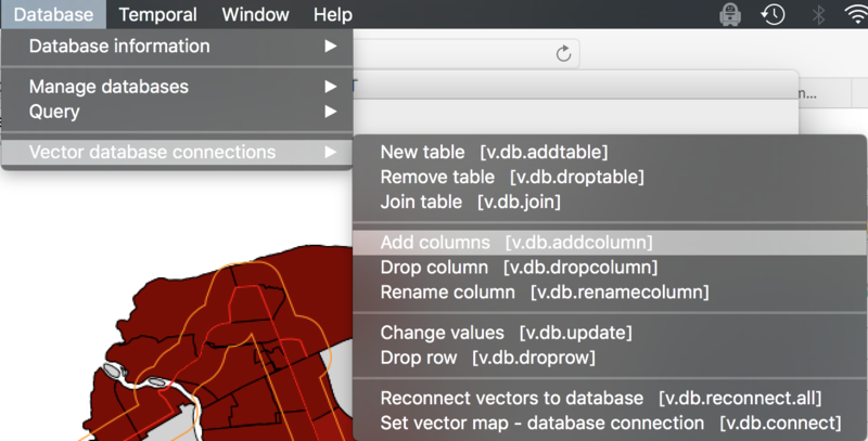
1. Click in the Database tab in the Grass GIS GUI and scroll down to Vector database connections and select the Add columns tool as seen in Figure 21.

Figure 21: Shows how to get to he add columns tool in the Grass GIS GUI.

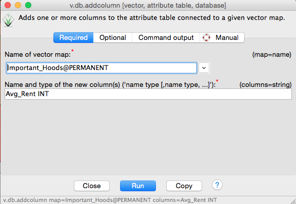
2. Once in the Add column window select the vector map you want to add data to. In this case our Important neighbourhoods layer. Then input the title of the new column, call this Avg_Rent and put INTafter so it is a column that will use integers. This can be seen in Figure 22.

Figure 22: Shows the input information to create an average rent column in the Important neighbourhoods vector map.

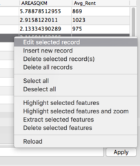
3. Go to the Ottawa Neighbourhood Study website and look up each of the neighbourhoods in the Important neighbourhoods vector map and find the average rent. Then go to the newly created average rent column and add the average rent to that column. This can be done by right clicking on the empty box and selecting Edit selected record, as shown in Figure 23.

Figure 23: How to edit a column in the attribute table.

Creating a Choropleth Map for Average Rent

Because Grass GIS 7.2 does not have a command that will allow it to create graduated symbols we will create a colour thematic map of average rent like we did for crime in step 5.9 Creating Choropleth Map for Crime. This will be done using the d.vect.thematic command like in step 5.9 but will call upon the Important neighbourhoods vector map and use different colours.

1. Input the following command into the Command Console:

d.vect.thematic -l map=Important_Hoods column=Avg__Rent algorithm=int nbclasses=5 colors="000:000:255,000:050:255,000:075:255, 000:100:255,000:125:255"

A new layer showing the average rents should appear and move from dark blue (Lower rent) to light blue (Higher rent).

2. Alternatively, you can use the Grass GUI Add thematic (choropleth) vector map function.

Creating the Final Maps

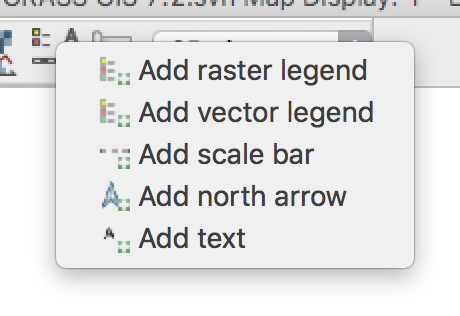
Final maps can be created by using the Add map feature button in the Grass GUI.

Figure 25: How to add final map features using the Grass GUI.

Conclusion

The usefulness of thematic mapping can go much farther than this specific application. Thematic mapping can show a variety of data in an easily interpretable manner. The project that was conducted in this tutorial is one such example that gets you to use the basic applications of working with vector maps and creating thematic maps. This project can also be improved upon with new data and refining of the current product.