Fire spread through cost path analysis in QGIS GRASS

Purpose

The purpose of this Wiki tutorial is to demonstrate a potential use of wildfire modeling tools in QGIS GRASS. The objective of this tutorial is to provide instructions on how to use digital elevation models (DEM) and vegetation data for setting up a cost analysis for wildfire spread in a given area. The process demonstrated in this tutorial would be able to be applied to different areas and different datasets.

Introduction

This tutorial will run using GRASS, an open source GIS software, which can be downloaded following the instructions in the next section. GRASS offers a range of tool-sets, including a Wildfire tool-set. This tutorial will run through a basic wildfire spread analysis in the Ottawa-Gatineau area, using some of the tools provided by the Wildfire tool-set.

We will be starting with two sets of data that were manipulated in ArcMap to be used for this tutorial. The first is a digital elevation model (DEM), and the second is a landcover type raster. DEMs can be used for many types of analysis, including hydrological or oceanography applications. In our case we will be using it to create wildfire spread analysis, by demonstrating cost paths in GRASS. Landcover is important to model the spread of fire, and so a raster was created to represent the landcover of the Ottawa region.

Materials and Data

GRASS is a free and open source geographic information system. The current stable version of GRASS is 7.2.2 , and can be downloaded as a stand-alone or as a package; we will be downloading it as a stand-alone. GRASS is available for a variety of platforms including Windows, Mac OS, and Linux. Various releases for download can be found at the GRASS website.

Before beginning this tutorial, both the landcover and elevation data were downloaded from Open Canada and then manipulated in ArcMap, prior to being imported into GRASS. These changes included, reducing the size of the data, creating our AOI, creating a custom symbology and customizing the projection in order to successfully import the data into GRASS.

The data required for this tutorial can be downloaded from:here.

Please ensure everything is downloaded before beginning the tutorial.

Methods

Setting up GRASS

This section will outline set up of the tutorial, preparing the data for manipulation in GRASS.

1. Launch GRASS

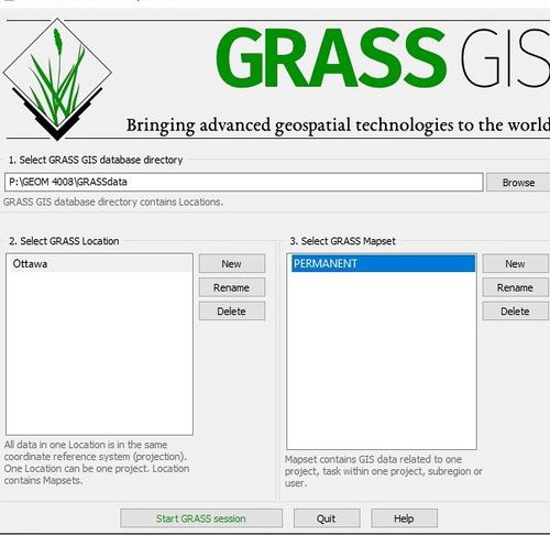
Figure 1. shows the setup needed for creating a GRASS project

Before starting the process, a GRASSdata folder is required; create a folder in the directory you want the project to be stored.

2. In the startup window, 'Browse' to and select the GRASSdata folder you created.

3. To select GRASS location, you must first create a new location. Click New and specify your project location. In our tutorial the project location is Ottawa. The rest of the fields are optional.

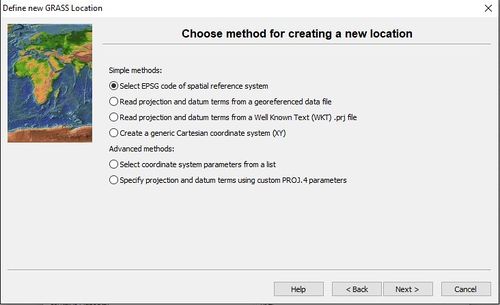
4. Choosing your method for creating a new location

Figure 2. Defining a new GRASS location

• Select the first method 'Select EPSG code of spatial reference system' and click Next. We are using this method because it allows us to match the location to our data's projection.

• In the 'Choose EPSG Code' window, search for the EPSG code: 4269 (NAD83). After selecting this projection, click Next. Another window will pop up, select default option and click OK, then finish.

5. In the startup window (Figure 1), Ottawa should now show in the location box. Single click the Location (Ottawa) and the new Mapset (PERMANENT), and click Start GRASS session.

Setting up the Data

1. You should now see the Layer Manager and Map Display windows open.

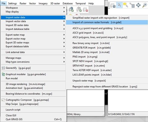
Figure 3. Pathway for importing raster data

• Import both rasters, as shown in Figure 3.
• In the r.in.gdal window, browse to the downloaded files, and select the aoi_complete_Project_Polygon2.tif file. Name the file 'Landcover',and click Run. Repeat this process for the OttawaDEM_Clip_ProjectRaster.tif file, and name it 'Elevation'.
• Both layers should now appear in the Layer Manager.

2. The next step is to set the symbology of the 'Landcover' layer. To do this, right click the 'Landcover' layer in the Layer Manager, and select Set color table interactively from the menu.

• In this window, select Clear all, and add twelve category values.
• Assign the twelve categories their respective number and colour based on the table below.

Table 1. Symbology of the Landcover raster data

Landcover type	Number	Colour
Mixedwood Dense	1	0:128:0
Mixedwood Open	2	0:244:0
Broadleaf Dense	3	0:64:40
Herb	4	128:128:64
Water	5	0:0:255
Coniferous Dense	6	0:47:0
Coniferous Open	7	82:119:26
Shrub	8	128:128:0
Broadleaf Open	9	0:170:0
Wetland	10	64:128:128
Cropland	11	186:186:116
Developed	12	255:128:192

3. Now we need to Set region under Computational region in the Settings dropdown menu from the GRASS GUI.

• Settings > Computational region > Set region
• In the Set region to match raster map(s): drop down, select the 'Landcover' layer.

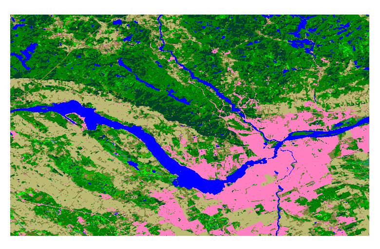
Your land cover symbology should look similar to this example below.

Figure 4. Landcover map output

Data Processing

Reclassify

This step is required to set up the data for the rate of spread tool in GRASS. This step reclassifies the landcover types into their hypothetical moisture values.

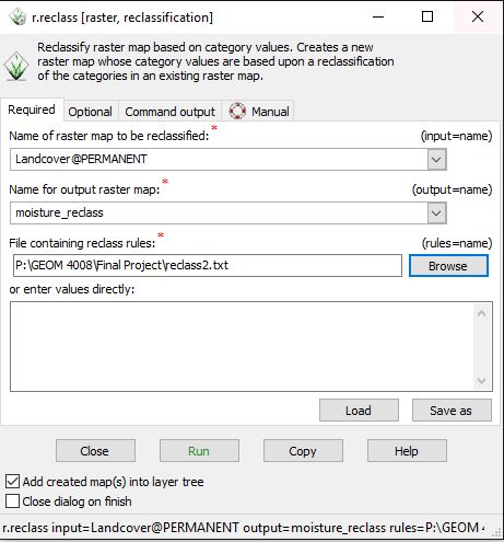
1. Navigate to r.reclass in the Raster dropdown menu, in the "Change category values and labels" tab.

• Raster > Change category values and labels > r.reclass

Figure 5. Reclass window

2. Select the 'Landcover' layer as your "Name of raster map to be reclassified:". Name the output as moisture_reclass.

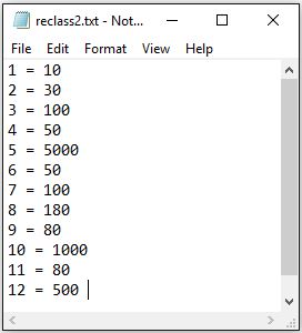
3. The next step requires a set of rules. The rules are required to set the parameters for the reclassification. This can be done in a text file, as shown in Figure 6.

Figure 6. Text document showing the rules

• The rules set the reclassification to specified numbers. In Figure 5, the 1-12 represents the different landcover types you classified in the above step. The numbers in the right column represent arbitrary values of moisture levels based on the given landcover.

This step creates a new layer.

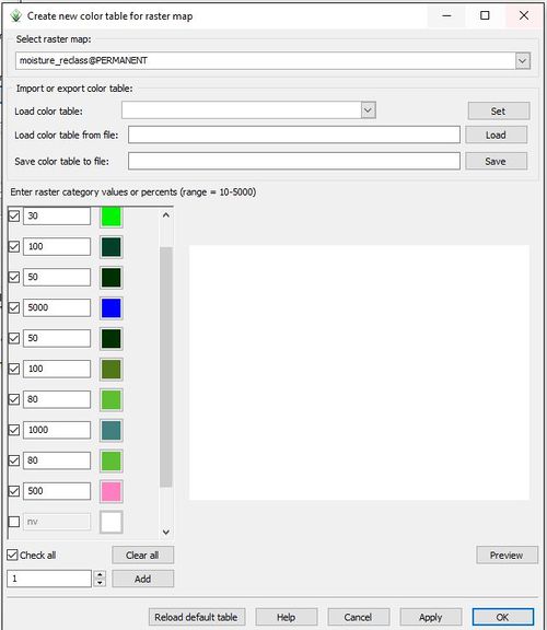
4. Right click the layer you created and go to the Set color table interactively tab.

Figure 7. Colour Table for reclassed layer

• Reduce the amount of category values to 12, and assign the moisture values from the rules text file. This is a similar process to the classification done above.
• Moisture levels that are the same will produce the same colour on the Map Display.

Raster Calculator

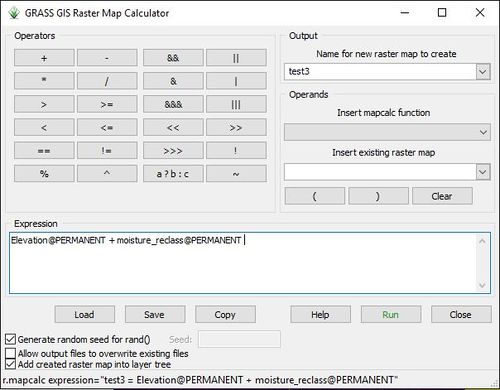
1. Open the Raster map calculator in the Raster drop down menu.

• Raster > Raster map calculator

Figure 8. Raster calculator window

2. Name your output map, and insert the elevation and moisture layers as seen in Figure 8.

Rate of Spread

The rate of spread tool (r.ros) generates four output raster map layers. These include:

• a base rate of spread
• a maximum rate of spread
• the direction of the maximum rate of spread
• the maximum potential spotting distance

Note: rate of spread needs to be run before the r.spread tool - these tools will later be combined in order to create a simulation of wildfire spread in the area.

Spread

The r.spread tool generates a raster map output of total spread time, given the rates of spread and direction of the rate of spread generated in the previous step.

Spread Path

1. After the r.ros and r.spread are generated, the r.spreadpath can be calculated.

2. The inputs for r.spreadpath will be the outputs you previously generated from the above steps.