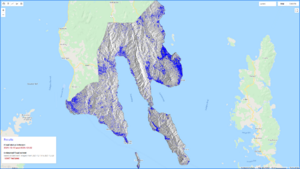
Flood Mapping and Area Calculation of Flood Extent Using Sentinel-I SAR Data in Google Earth Engine: the case of Super Typhoon Odette (Rai)
Contents
- 1 Introduction
- 2 Setting up Google Earth Engine
- 3 Tutorial
- 3.1 Preparing your data
- 3.2 Step 1. Selection of Study Area
- 3.3 Step 2. Setting the time frame
- 3.4 Step 3. Selection of Sensor Parameters
- 3.5 Step 4. Area calculation of flood extent
- 3.6 Step 5. Running the script
- 3.7 Step 6. Visualizing Results in Google Earth Engine
- 3.8 Step 7. Exporting generated products
- 4 Conclusion
- 5 References
Introduction
Purpose and Overview
This tutorial aims to produce a map showing the flood extent of the affected areas. This can be achieved by building scripts to gather satellite images taken before and after a flood event and comparing them. Google Earth Engine provides large-scale visualization and analysis of geospatial data, particularly Sentinel-I SAR GRD imagery. This approach is used due to its resistance to weather and cloud cover; thus, it is a reliable way to detect flooded regions.
Google Earth Engine (GEE) is a free, planetary-scale platform software used for educational and operational research and non-profit use. This open software developed by Google has been used to operate various studies on a global and regional scale, including Land Use and Land Cover (LULC), flood mapping, surface water mapping, and other applications.
Flood mapping is important especially in tropical regions because these areas are prone to typhoons and cyclones and are usually surrounded by open waters. This is crucial during the immediate response phase to make decisions on evacuations, calculating the extent of damages, and appropriate deployment of aid for the victims.
Area of Interest
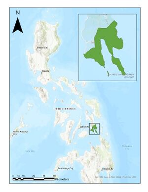
On December 16, 2021, a super typhoon Odette or Rai, as named internationally, severely affected the Visayas and Mindanao group of islands in the Philippines. This typhoon fell on a Category-5 scale and was considered as one of the strongest storms that struck the country.
In this tutorial, the area of interest will be in the province of Southern Leyte, located in the Eastern Visayas Region of the Philippines. This area is chosen because there were not a lot of GIS articles written about this phenomenon, since it only occurred a week ago. In this way, the flood extent of Southern Leyte will be determined while learning how to generate it using Google Earth Engine.
Setting up Google Earth Engine
Google Earth Engine is a web-based integrated development environment (IDE) for JavaScript API and a cloud-based geospatial procession platform. To make sure that working in this software is fast and easy, you should have a Google Earth Engine account.
Creating an account
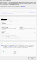
- Go to https://signup.earthengine.google.com/ and sign up with your Google account. You can also use your existing Gmail account to sign-up.
Note: This step usually takes 1 - 2 days for approval. Do this as soon as possible.
- After approval, you will receive an email from Google to confirm that you are all set up.
- Then, go to https://code.earthengine.google.com/ to start coding!
To ensure a hassle-free sign-up process, follow these tips:
- Use Google Chrome browser.
- If you have multiple Google accounts, make sure that you are logged in to the account that you want to be associated with Earth Engine.
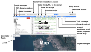
Components of Google Earth Engine Code Editor
You should have a stable internet connection and some storage left in your Google Drive depending on the size of your study area. After going to the website, you should see the entire components of the Earth Engine Code Editor:
Setting up your repository
You need to create your Owner repository folder to be able to save your codes and files. To do this:
- Click the NEW button on the right side of the editor.
- Click Repository.
- Write a repository name of your choice. It must be unique, and you cannot change it later.
- When you save your scripts later, they will be saved under the Owner section.
Tutorial
Preparing your data
To prepare your data, follow these steps:
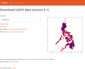
- Download the shapefile of the Philippine administrative area in GADM here.
- Choose Philippines in the country drop-down menu.
- Click Shapefile. The zip file download will start automatically.
- In your Downloads file location, extract the zip file into a different folder by right-clicking it and choosing Extract to gadm41_PHL_shp/. There should be a folder in the same location.
Note: You will only need Level 1 shapefiles for this tutorial.
Step 1. Selection of Study Area
This information is vital to limit the extent of the analysis and avoid unnecessary calculations. In this tutorial, we will be focusing on the provincial boundary of Southern Leyte, Philippines. There are a few ways to specify the location of your study area (polygon tool or GEE FeatureCollection) and uploading a shapefile (.shp) is the most accurate solution.
Note: Make sure to include .dbx and .shx files because your shapefile depends on them.
To upload the shapefiles that you downloaded earlier:
- Go to Assets tab on the left side of the Code Editor.
- Click NEW, and select Shape Files.
- Click SELECT, and go to the location of the extracted folder named gadm41_PHL_shp.
- Hold the Ctrl button on your keyboard, and choose three files: gadm41_PHL_1.dbf, gadm41_PHL_1.shp, and gadm41_PHL_1.shx and click Open.
- Create an optional name for these files under Asset ID. This can be helpful to easily recognize your uploaded files. However, for this tutorial, we will name it PH_Lev1.
- Then click UPLOAD.
Uploading this file may take a few minutes. You can check the status of the upload by clicking the Tasks tab on the right panel of the Code Editor. The “Ingest Table” will turn blue when it is complete.
- Before writing your first script, click NEW on the right panel of the editor and choose FILE. Create your file name and select OK. Whenever you make changes to your script, do not forget to hit SAVE at the top of the editor to save your work.
- Import the file to the script by clicking the Assets tab on the left panel, and under your username, you should be able to find the uploaded shapefile.
- Hover your mouse on the PH_Lev1, and on the rightmost side, you will see a small arrow that indicates “Import into script”. Click that arrow.
- After importing the file, click this icon
 found in your code editor, and copy and paste the generated code in the empty code editor.
- Replace the word table with admin. It should be like this:
Note: The yourname section in the code depends on your username. Do not copy it.
var admin = ee.FeatureCollection("users/yourname/PH_Lev1");
- Since we only need the province of Southern Leyte, a filtering function should be applied. Use the code below:
var geometry=admin.filter(ee.Filter.eq('NAME_1','Southern Leyte'));
- Then generate a map with your desired colour. For this tutorial, we will use the colour grey. Use the code below:
Map.addLayer(geometry,{color:'grey'},'Southern Leyte');
- Finally, click Run, and you can see that your map section has been highlighted into grey colour. You can zoom on it as this indicates your study area.
Step 2. Setting the time frame
Other than the area of interest, you are also required to define the dates of pre-flood and post-flood periods on the next script. To compare the two images, you should indicate the periods before the flood, and the periods after the flood. Sentinel-1 imagery requires 6-12 days on each time period. In this tutorial, our pre-flood dates will be from November 15, 2021, to December 14, 2021, and the post-flood dates are from December 15, 2021, to December 22, 2021.
Note: The date formatting for the script should be YYYY-MM-DD (if you want to change the time period).
Set the time frame by copying this code:
var before_start= '2021-11-15';
var before_end='2021-12-14';

var after_start='2021-12-15';
var after_end='2021-12-22';
Step 3. Selection of Sensor Parameters
Next, we need to set the sensor parameters by choosing the polarization between VH and VV or both to perform the analysis. VH is highly recommended for flood mapping because it is more susceptible to any changes on the land surface, while VV is more useful for open waters from the land surface like shoreline detection. In this tutorial, we will be using both VV and VH because the province of Southern Leyte is also located in a coastal area. Use the code below:
var polarization = ("VH","VV");
Another parameter is change detection. This is important to select the same pass direction of the images being compared and avoid wrong signals because of the difference in the viewing angle. Revisit this page, and you can see that the Philippines is only covered by DESCENDING pass direction. Therefore, indicate this by writing this code:
var pass_direction = "DESCENDING";
Applying a threshold is another necessary parameter to extract the difference between the pre-flood and post-flood images. We have set the threshold to 1.00, so any pixel that is greater than 1.00 difference is considered as a flooded area. Indicate this in the script by typing this code:
var difference_threshold = 1.00;
Next, you will load and filter Sentinel-1 GRD imagery data from the parameters you have set above. Aside from them, you also need to gather the images by the dates you have indicated at the beginning of your script. To proceed, rename the selected geometry feature first to indicate your area of interest. Do this by copying these codes:
var aoi=geometry;
var collection= ee.ImageCollection('COPERNICUS/S1_GRD')
  .filter(ee.Filter.eq('instrumentMode','IW'))
  .filter(ee.Filter.listContains('transmitterReceiverPolarisation', polarization))
  .filter(ee.Filter.eq('orbitProperties_pass',pass_direction))
  .filter(ee.Filter.eq('resolution_meters',10))
  .filterBounds(aoi)
  .select(polarization);
var before_collection = collection.filterDate(before_start, before_end);
var after_collection = collection.filterDate(after_start,after_end);
function dates(imgcol){
        var range = imgcol.reduceColumns(ee.Reducer.minMax(), ["system:time_start"]);
        var printed = ee.String('from ')
          .cat(ee.Date(range.get('min')).format('YYYY-MM-dd'))
          .cat(' to ')
          .cat(ee.Date(range.get('max')).format('YYYY-MM-dd'));
        return printed;
      }
      // print dates of before images to console
      var before_count = before_collection.size();
      print(ee.String('Tiles selected: Before Flood ').cat('(').cat(before_count).cat(')'),
        dates(before_collection), before_collection);

      // print dates of after images to console
      var after_count = before_collection.size();
      print(ee.String('Tiles selected: After Flood ').cat('(').cat(after_count).cat(')'),
        dates(after_collection), after_collection);

// Create a mosaic of selected tiles and clip to study area
var before = before_collection.mosaic().clip(aoi);
var after = after_collection.mosaic().clip(aoi);

// Apply reduce the radar speckle by smoothing
var smoothing_radius = 50;
var before_filtered = before.focal_mean(smoothing_radius, 'circle', 'meters');
var after_filtered = after.focal_mean(smoothing_radius, 'circle', 'meters');
Step 4. Area calculation of flood extent
After setting the parameters inside the area of interest, you will now proceed to calculate the area of the flood extent. Having visual and numerical measurements on this data will give you a basic understanding of how serious the flood was. Follow this code to proceed with the area calculation. The results will be displayed on the "Results" panel in the bottom-left corner of the Map Viewer after you Run the script.
// Calculate the difference between the before and after images
var difference = after_filtered.divide(before_filtered);

// Apply the predefined difference-threshold and create the flood extent mask
var threshold = difference_threshold;
var difference_binary = difference.gt(threshold);

// Refine flood result using additional datasets

      // Include JRC layer on surface water seasonality to mask flood pixels from areas
      // of "permanent" water (where there is water > 10 months of the year)
      var swater = ee.Image('JRC/GSW1_0/GlobalSurfaceWater').select('seasonality');
      var swater_mask = swater.gte(10).updateMask(swater.gte(10));

      // Flooded layer where perennial water bodies (water > 10 mo/yr) is assigned a 0 value
      var flooded_mask = difference_binary.where(swater_mask,0);
      // final flooded area without pixels in perennial waterbodies
      var flooded = flooded_mask.updateMask(flooded_mask);

      // Compute connectivity of pixels to eliminate those connected to 8 or fewer neighbours
      // This operation reduces noise of the flood extent product
      var connections = flooded.connectedPixelCount();
      var flooded = flooded.updateMask(connections.gte(8));

      // Mask out areas with more than 5 percent slope using a Digital Elevation Model
      var DEM = ee.Image('WWF/HydroSHEDS/03VFDEM');
      var terrain = ee.Algorithms.Terrain(DEM);
      var slope = terrain.select('slope');
      var flooded = flooded.updateMask(slope.lt(5));

// Calculate flood extent area
// Create a raster layer containing the area information of each pixel
var flood_pixelarea = flooded.select(polarization)
  .multiply(ee.Image.pixelArea());

// Sum the areas of flooded pixels
// default is set to 'bestEffort: true' in order to reduce computation time, for a more
// accurate result set bestEffort to false and increase 'maxPixels'.
var flood_stats = flood_pixelarea.reduceRegion({
  reducer: ee.Reducer.sum(),
  geometry: aoi,
  scale: 10, // native resolution
  //maxPixels: 1e9,
  bestEffort: true
  });

// Convert the flood extent to hectares (area calculations are originally given in meters)
var flood_area_ha = flood_stats
  .getNumber(polarization)
  .divide(10000)
  .round();
Step 5. Running the script
When the area of interest is selected and all parameters are determined, click RUN and wait for a few minutes. You can see the area of interest is highlighted in the map section. The parameters are not visualized yet.
Step 6. Visualizing Results in Google Earth Engine
This section lets you write a script to display the results on the map. There will be a panel where the results will be shown including the estimated flood extent area from the calculation above. To do this, follow the code below:
// Set position of panel where the results will be displayed
var results = ui.Panel({
  style: {
    position: 'bottom-left',
    padding: '8px 15px',
    width: '350px'
  }
});

// Prepare the visualization parameters of the labels
var textVis = {
  'margin':'0px 8px 2px 0px',
  'fontWeight':'bold'
  };
var numberVIS = {
  'margin':'0px 0px 15px 0px',
  'color':'bf0f19',
  'fontWeight':'bold'
  };
var subTextVis = {
  'margin':'0px 0px 2px 0px',
  'fontSize':'12px',
  'color':'grey'
  };

var titleTextVis = {
  'margin':'0px 0px 15px 0px',
  'fontSize': '18px',
  'font-weight':'',
  'color': '3333ff'
  };

// Create labels of the results
// Title and time period
var title = ui.Label('Results', titleTextVis);
var text1 = ui.Label('Flood status between:',textVis);
var number1 = ui.Label(after_start.concat(" and ",after_end),numberVIS);

// Alternatively, print dates of the selected tiles
//var number1 = ui.Label('Please wait...',numberVIS);
//(after_collection).evaluate(function(val){number1.setValue(val)}),numberVIS;

// Estimated flood extent
var text2 = ui.Label('Estimated flood extent:',textVis);
var text2_2 = ui.Label('Please wait...',subTextVis);
dates(after_collection).evaluate(function(val){text2_2.setValue('based on Sentinel-1 imagery '+val)});
var number2 = ui.Label('Please wait...',numberVIS);
flood_area_ha.evaluate(function(val){number2.setValue(val+' hectares')}),numberVIS;

results.add(ui.Panel([
        title,
        text1,
        number1,
        text2,
        text2_2,
        number2,
       ]
      ));
Map.add(results);

// Before and after flood SAR mosaic
Map.centerObject(aoi,8);
Map.addLayer(before_filtered, {min:-25,max:0}, 'Before Flood',0);
Map.addLayer(after_filtered, {min:-25,max:0}, 'After Flood',1);

// Difference layer
Map.addLayer(difference,{min:0,max:2},"Difference Layer",0);

// Flooded areas
Map.addLayer(flooded,{palette:"0000FF"},'Flooded areas');
- When you hit "Run" after these scripts, you can see the changes in the Map Section, along with the results panel.
- Click the Layers button to change the visibility of the layers by checking or unchecking them.
- To view the full map in full-screen, select the full-screen button at the top right corner of the map viewer.
- Once you are all done with your script, click SAVE to save your work under the file name you created.
Step 7. Exporting generated products
Exporting the generated layers from your scripts lets you save the raster or vector images on your Google Drive account so that you can use them outside the platform. To do this, first copy this code:
 // Export Flood Extent Raster
var projection = after_collection.first().projection().getInfo() // This gets the projection for the aoi
Export.image.toDrive({
  image: flooded,
  description: 'Flood_extent_raster',
  crs: projection.crs,
  crsTransform: projection.transform,
  region: geometry
});
- Click on the TASKS tab located at the right side of the code editor.
- There should be a product generated there. Flood_extent_raster produces a GeoTIFF raster file of the flood extent. This raster file can be used in other software such as QGIS or ArcGIS to produce a vector shapefile for further analysis.
- Choose the generated output you want to export and click RUN.
- On the pop-up window, it will ask you to type in your personalized filename, where to save it, and the format you prefer. Saving it in your Google Drive account is the easiest way. When you are all set up, click RUN.
- Go to your Google Drive account and you should see the file name or file folder you have created.
Conclusion
Google Earth Engine is a powerful web platform for cloud-based data processing of remote sensing data on global scales. It has a wide variety of data catalogues that you can use for any other uses such as flood mapping and damage assessment. This Wiki tutorial is only one of many operations this tool can perform. This is a recommended practice for beginners and intermediate users of Google Earth Engine because it is less complicated and there are numerous guides and codes online that can be copied and pasted because it uses a common programming language, JavaScript.
References
- Earth Engine Code Editor | Google Earth Engine | Google Developers. (n.d.). Retrieved December 23, 2021, from https://developers.google.com/earth-engine/guides/playground
- GADM. (2021). Global Administrative Areas. https://gadm.org/download_country.html
- Mehmood, H., Conway, C., & Perera, D. (2021). Mapping of Flood Areas Using Landsat with Google Earth Engine Cloud Platform. Atmosphere, 12(7), 866. https://doi.org/10.3390/atmos12070866
- Recommended Practice: Flood Mapping and Damage Assessment Using Sentinel-1 SAR Data in Google Earth Engine | UN-SPIDER Knowledge Portal. (n.d.). Retrieved December 23, 2021, from https://www.un-spider.org/advisory-support/recommended-practices/recommended-practice-google-earth-engine-flood-mapping
- Super Typhoon Rai’s Death Toll in Philippines Is Climbing—The New York Times. (n.d.). Retrieved December 23, 2021, from https://www.nytimes.com/2021/12/19/world/asia/philippines-super-typhoon-rai-odette.html
