Flood Risk Assessment in QGIS
Contents
Introduction
Flood assessment is one of many important purposes for which GIS capabilities can be applied in a practical manner. The scope of the analysis in the tutorial includes a portion of the downtown core of Ottawa, ON. This analysis is particularly relevant due to the high number of flooding events and high-rainfall in Ottawa, especially in 2017. By completing flood risk assessments the city can identify at-risk buildings/populations, as well as develop stronger preparedness measures for when a flood does occur.
The purpose of this tutorial is to provide users with an introduction/guidance in completing a flood risk assessment. The software that will be used is QGIS (ver. 2.18.10) as well as ArcMap (ver. 10.5.1) solely for preliminary data processing.
Data and Software Requirements
In order to begin this tutorial a download of the QGIS software is needed. The current version is QGIS 2.18.15 'Las Palmas' and was released on 08.12.2017. QGIS is available on Windows, MacOS X, Linux as well as Android. This can be found at QGIS Download
Moving forward, the elevation data that will be used for this tutorial can be found from this link. For the purpose of this analysis, 4 adjacent elevation tiles of the city of Ottawa were downloaded, which make a 4-tiled square. Be sure to download the files as shapefiles, not DEMs.
You may use whatever additional base layers you might like to add to this tutorial, but for this purpose, only roads, buildings, and water body data is used which can be found here In addition to the major waterways, roads and building data, this dataset also provides contours, airports, railroads, etc.; but for the purpose of this tutorial, please use ‘Major_Water.shp’; ‘Roads.shp’; and ‘Buildings.shp’.
After all the data is downloaded, you may proceed to process the files in ArcMap.
ArcMap Processing
In order to create the proper DEM file needed to process the desired outcome of this tutorial, the four grid files previously mentioned must be loaded into ArcMap and then processed into DEMs using the Spatial Analyst tool: Inverse Distance Weighted (or IDW for short).
We used ArcMap as a tool to process the data into a file type that QGIS would recognize and be used for the computation/analysis processes.
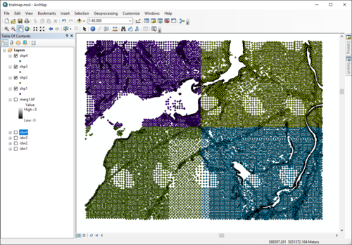
Step 1. Import the four shapefiles that were downloaded through the Carleton Library. Your screen should look something similar to this image
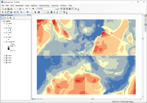
Step 2. Convert the shapefiles to raster using the IDW tool. The result should look very similar to this image
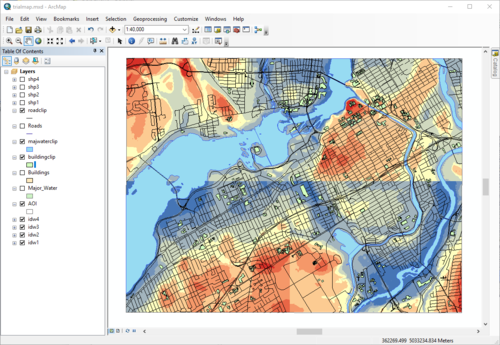
Step 3. Clipping, Major Water, Roads, Buildings Used an AOI polygon feature, that was set to the same extent as the IDW tiles, to clip features. → you can also clip the data in QGIS, but to streamline the process in QGIS, we clipped the data in ArcMap. The result should look similar to this image
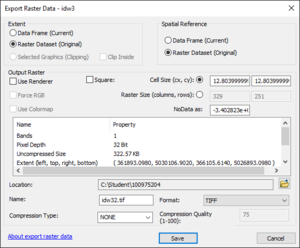
Step 4. Export the IDW raster files into a .tif This should be the window that appears after selecting the export data option from right-clicking on the layer file.
QGIS Methods
Merging
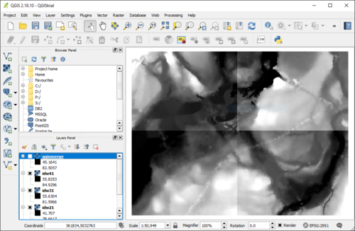
Step 1. Upload the .tif files into QGIS and you should see a result similar to this one:
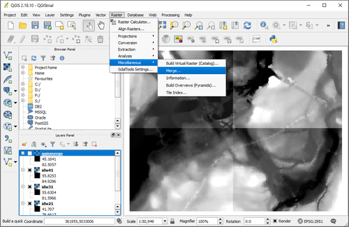
Step 2. Use the merge tool to combine the .tif files into one working layer feature. The merge tool can be found under the raster menu under miscellaneous as seen below
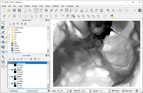
The result should look similar to this image
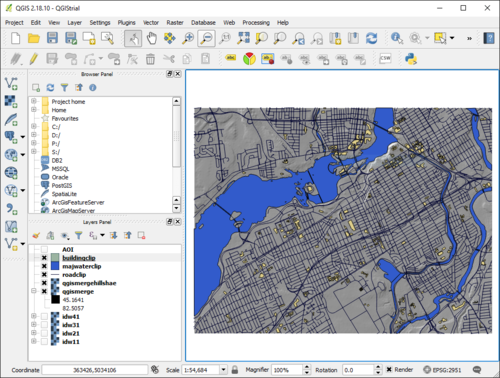
Step 3. Once the final raster has been created the new clipped polygons; Roads, Major Water, and Buildings (from ArcMap) can be added into QGIS. After the following two steps and some colour alterations (based on personal preferance) the result should look very similar to this image
Sink Fill
Step 4. Sink Fill (Wang & Liu) was used from the QGIS toolbox. This was used in order to fill any spatial outliers that may have an effect on the overall result of the flood risk assessment.
Raster Calculator
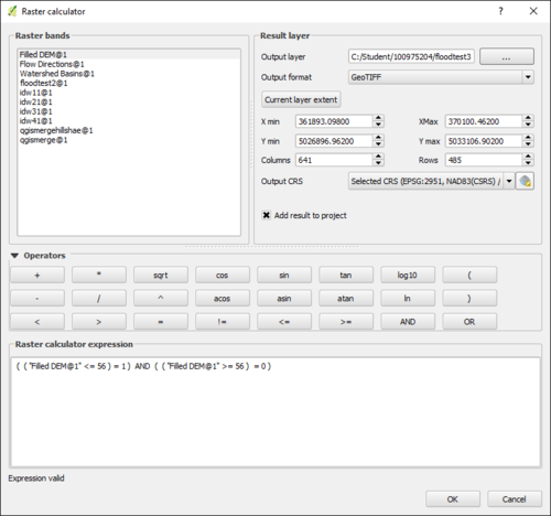
Step 5. Raster Calculator to establish what areas will be flooded given an increase of water level; visualized in our example is an increased water level of 1m. The following was inputted into the command box:
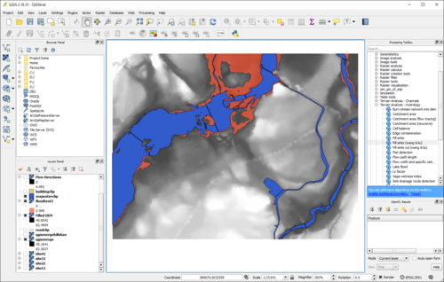
The result after some color alterations once again should look like this image below
- Note: 1:100 stormwater approx 100mm/24hr period based on the link below
