Difference between revisions of "Georeferencing Raster Imagery in QGIS using Vector Data"
| Line 12: | Line 12: | ||
==Acquiring Data== |
==Acquiring Data== |
||
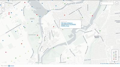
| − | Before beginning to aquire the data necessary for this exercise, it is best to create a folder to organize all of your project elements into. Somewhere on your computer that is easy to access (preferably in your C: drive on windows, or HOME directory on Linux), create a folder named ''Georeferencing Exercise'''. This will be the location where we store all our data, as well as the QGIS project files. [[File:photoLocation.png|400px|thumb|right|Location of 1933 air photo used in this tutorial]] |
+ | Before beginning to aquire the data necessary for this exercise, it is best to create a folder to organize all of your project elements into. Somewhere on your computer that is easy to access (preferably in your C: drive on windows, or HOME directory on Linux), create a folder named ''Georeferencing Exercise'''. This will be the location where we store all our data, as well as the QGIS project files. [[File:photoLocation.png|400px|thumb|right|Figure 2: Location of 1933 air photo used in this tutorial]] |
The air photo used for this example can be located here: [https://library.carleton.ca/find/gis/geospatial-data/carleton-campus-aerial-images]. At this link, scroll about a third of the way down to the section labelled '''Available Themes'''. Select the bottom-most link '''1930s - 1945 air photos from uOttawa'''. Refer to the figure on the right of this section of the tutorial to visualize the location of the desired photo. Click the dot, then the link that appears. Once on a screen with the photo as per figure, right click the photo and select ''Save Image As...''. Save it to the folder made earlier. |
The air photo used for this example can be located here: [https://library.carleton.ca/find/gis/geospatial-data/carleton-campus-aerial-images]. At this link, scroll about a third of the way down to the section labelled '''Available Themes'''. Select the bottom-most link '''1930s - 1945 air photos from uOttawa'''. Refer to the figure on the right of this section of the tutorial to visualize the location of the desired photo. Click the dot, then the link that appears. Once on a screen with the photo as per figure, right click the photo and select ''Save Image As...''. Save it to the folder made earlier. |
||
Revision as of 16:49, 2 October 2019
Contents
- 1 Purpose
- 2 Introduction
- 3 Acquiring Data
- 4 Installation of QGIS
- 5 Adding Reference Vector Data into QGIS
- 6 Accessing the Georeferencing Plugin
- 7 Using Georeferencer GDAL
- 8 References
Purpose
The purpose of this tutorial is to learn how to conduct a georeferencing process on a non-georeferenced air photo in QGIS. In doing so, you will also gain knowledge on navigating through, and working with, the QGIS environment. For the purpose of this tutorial, a basic understanding of GIS is assumed.
Introduction
QGIS: An Introduction
QGIS is an open-source GIS Software initially created in 2007 as Quantum GIS by the Open Source Geospatial Founndation. Open-source means the program is free to use, and the code used to make it is freely accessible. The software GUI contains many of the same geoprocessing and cartographic tools as well-known ArcGIS, along with an extensive Python library that can be used to automate processing. Other open-source software packages are also integrated into the QGIS environment, such as: SQLite, GDAL, PostGIS and PostgreSQL, while others such as GRASS and MapServer work directing in conjunction with QGIS. The programs runs on Mac OS, Linux, UNIX, Android, and Microsoft Windows.
Georeferencing
When data is collected via a remote sensing platform, whether that be a camera in a plane, or a thermal sensor in a satellite, the data collected must be aligned to real-world locations in order to be useful. Geo-referencing in GIS allows the user to do just this, using a known coordinate system and known points on the ground to align remotely sensed data so that it may be viewed, queried or analyzed with other geospatial data. These reference points are known as ground control points, or GCPs, and are stored in the metadata of .tif raster files once created. Creating GCP's to align the datasets will often manipulate the data set by shifting, scaling, rotating or skewing.
Acquiring Data
Before beginning to aquire the data necessary for this exercise, it is best to create a folder to organize all of your project elements into. Somewhere on your computer that is easy to access (preferably in your C: drive on windows, or HOME directory on Linux), create a folder named Georeferencing Exercise'. This will be the location where we store all our data, as well as the QGIS project files.
The air photo used for this example can be located here: [1]. At this link, scroll about a third of the way down to the section labelled Available Themes. Select the bottom-most link 1930s - 1945 air photos from uOttawa. Refer to the figure on the right of this section of the tutorial to visualize the location of the desired photo. Click the dot, then the link that appears. Once on a screen with the photo as per figure, right click the photo and select Save Image As.... Save it to the folder made earlier.
In terms of reference vector data, study the image selected and locate as much reference vectore data as possible. This includes roads [2] (select Roads and Sidewalks under Ottawa-Gatineau section of this page), the railway line [3] (Select Direct Download - Carleton University campus datasets, followed by Construction_Services_GIS/, then rail.ZIP), and the river [4]. Download these three vector datasets, and extract them into your project folder made earlier.
Since this particular photo was taken in 1933, there will be sections of the data that do not exist in the image, but do not let this discourage you, as the sections that do will still be accurate, though created over 80 years later.
Installation of QGIS
You can download QGIS from the following link [5] using the green Download Now button. Choose your platform: Windows, Mac OS X, Linux, BSD, or Android from the various drop-down menus on the download page (Windows will be used for this tutorial. If you have Windows, check your specifications and either you will use 32 bit or 64 bit. Select the latest standalone version and download the .exe istaller. Once downloaded, go to the location the .exe installer downloaded to, run it, and use the Setup Wizard that appears to configure the program.
Once QGIS is fully installed onto your computer, run it either via the desktop icon, or the start-menu launcher. Once opened, a program window like figure should appear. To create a project file for our project, click Project in the upper left corner, and Save As. Browse to the folder created in the earlier step, give the project a name, like Georeferencing Tutorial, and hit Save.
Adding Reference Vector Data into QGIS
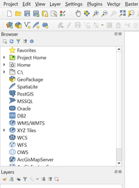
The easiest way to add our reference vector data into the QGIS is by using the Browser. On the middle-left, as per figure is a window containing various programs data can be added from. We are most concerned with the Project Home link near the top of this section. Click the drop down arrow to the left of this label. You should notice all of the vector files downloaded earlier listed here. Double-click the rails.shp, RoadsSidewalks_polygon_MTM9.shp, and Water.shp files to add them to our QGIS session. If by happenstance your vector files are not in Project Home, simply browse to where you unzipped your vector data via the drop-downs from your main hard drive, in the case of Windows, C:/.
Accessing the Georeferencing Plugin
The georeferencing tool in QGIS comes installed with the program, but is not visible by default. To use it, we must activate the plugin.
- To access the plugins manager, select Manage Plugins under the Plugins drop-down menu on the main tool bar.
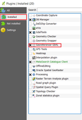
- A window will open providing you with several options for plugins, navigate to the Installed subsection as per Figure 14
- Toggle the Georeferencer GDAL plugin, and close this menu.
Using Georeferencer GDAL
Now that the Georeferencer plugin is active and our vector data is loaded in QGIS, we can begin to add GCPs to our non-georeferenced .jpg file.
Opening the Georeferencer
Navigate to the main toolbar, and select the Raster Menu. You will notice that Georeferencer can be found at the bottom of the menu. Open the Georeferencer...
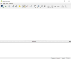
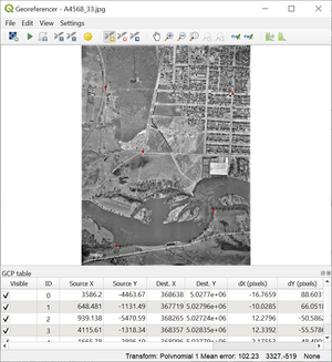
The Georeferencer window will appear separate from the main GUI, and will look like the figure to the right. It is recommended that both windows be viewed at the same time, so split them across your desktop as best as possible.
Adding a Raster
Navigate to the main toolbar in the Georeferencer window and select the Add Raster Layer icon. Navigate to the location of our non-georeferenced .jpg file and add it to the window.
Zooming In and Out
- To zoom in on the image in the georeferencer window select the Zoom In icon.

- To zoom out on the image in the georeferencer window select the Zoom Out icon.

- To move around the image, select the Pan icon

Adding Control Points
If you already have control points saved, you can load the file by selecting the Load Points icon ![]() Otherwise…
Otherwise…
Select the add control point icon .
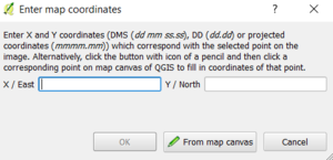
- A window will appear prompting you to add the coordinates of the point, or find it on the referenced file within the main window of QGIS.
- If you know the coordinates, enter them. Otherwise select From Map Canvas. This will minimize the georeferencer window, leaving the main QGIS window with the vector data opened earlier. Click the location on the vector data that corresponds to the same location in our image. This will save the point as a GCP.
- To delete a point, select the Delete Point icon

- You can move points by selecting the Move Points icon on the toolbar.

Add the first 4-5 GCPs across the entirety of the image, as per figure _.
This is to prevent the image from being warped more to one side. Continue to the next steps will these GCPs, as we can come back later to add more if needed.
Points Table
- The points which you have placed on your map image will appear below the raster image in the window.
- To save your points select the Save Points icon on the toolbar.

- This will save your points to an .aux.xml file for later viewing, or to add back into the Georeferencer.
- If the residuals are high for some of your points, you should go back and move the point to be more accurate.
Transformation Settings
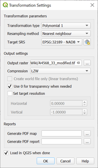
To access the transformation settings navigate to the toolbar on the Georeferencer and select the Transformation Settings icon. ![]()
After adding the Geographic Control Points (GCPs) you will need to define the settings for the georeferencing procedure.
- Depending on how many points you have added to your image you may want to choose different transformation algorithms for your image.
Transformation Type
Choose an appropriate transformation type.
- The transformation types available to you include:
- Linear: This is used to generate a world-file that will be different from the other algorithms available because it does not actually transform your image. This probably won't be the best option if you are using scanned imagery.
- Helmert: This transformation will run simple scaling and rotation transformations.
- Polynomial Algorithms: These will match source and destination control points. The 2nd order polynomial transformation allows for some curvature in your transformation. Using a 1st order polynomial transformation (affine) will perserve collinearity and will only permit scaling, translation and rotation on the image.
- Thin Plate Spline: This transformation is able to introduce local deformations in the data. This is good if the original image being georeferenced is of poor quality.
- Projective: The projective transformation is a linear rotation and translation of coordinates.
Defining the Resampling Method
- Select one of the resampling method options by clicking on the drop down list. Your choice will vary depending on the objectives of your task.
- Choose one of the following options:
- Nearest neighbour
- Linear
- Cubic
- Cubic Spline
- Lanczos
Compression
- Select the type of compression you wish to occur on your image.
- The options include:
- NONE
- LZW
- PACKBITS
- DEFLATE
Output Raster
- Select the name and location for the output file by selecting the Output Raster icon, navigating to the appropriate folder and providing a name.
Target Spatial Reference System (SRS)
- Choose the target coordinate system for your raster image by clicking the Target SRS icon [[6]]
- A window will appear prompting you to choose a coordinate system for your image.
Generating a pdf map and report
- To save a map or report to disk as a .pdf file, select the .pdf document icon next to Generate pdf map and/or Generate pdf report.
- Navigate to the appropriate directory to save your files.
Set Target Resolution
Toggle on Set Target Resolution to set a custom pixel resolution for your output raster.
Additional Options
- Toggle on Use 0 for transparency when needed to make areas with the value of 0 transparent.
- Toggle on Load in QGIS when done to add the image into QGIS as a layer whenever the georeferencing process is complete.
- Toggle on Create world file for linear transformations.
For this example, the settings used can be found in figure_, the output filename can be whatever you like. Once all the settings are selected, select OK when complete.
Running the Georeferencer
Once all of the GCPs have been added and the Transformation Settings have been selected you can now georeference your raster image.
- Select the Start Georeferencing icon on the main toolbar.

- Make sure to check the box to add the image to your project.
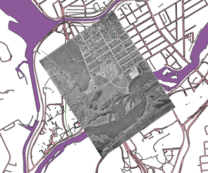
- This will create a new georeferenced image.
Your end resultant should look something like figure _. If you want to add more GCPs to make your georeferenced image even more accurate, just go back to the Georeferencer window, reference more GCPs, and run the georeferencer again!
References
52°North Initiative for Geospatial Open Source Software. (2013). ILWIS Open. Retrieved December 10, 2013, from 52°North: http://52north.org/communities/ilwis/ilwis-open
esri. (2013). GIS Dictionary. Retrieved December 10, 2013, from esri support: http://support.esri.com/en/knowledgebase/GISDictionary/term/vector
ESRI. (2008, September 22). What is a raster data? Retrieved December 10, 2013, from ArcGIS 9.2 Desktop Help: http://webhelp.esri.com/arcgisdesktop/9.2/index.cfm?TopicName=What_is_raster_data%3F
Geomatics Solutions. (2011). NAD83 / MTM zone 9. Retrieved 2013, from Georepository: http://georepository.com/crs_32189/NAD83-MTM-zone-9.html
GNU. (2013, September 12). GNU General Public License. Retrieved December 10, 2013, from GNU Operating System : https://gnu.org/licenses/gpl.html
Python Software Foundation. (2013). Python Programming Language – Official Website. Retrieved December 10, 2013, from Python: http://python.org

