Hazardous Areas Around Linear Infrastructure

Introduction

Introduction Mountainous terrain can pose challenges for linear infrastructure such as railway lines and highways. Not only do such areas present operational challenges, they also pose risks due to mass movements such as landslides, rock slides, and avalanches that can lead to physical damage, temporary closure, and even loss of life. Having information on potential locations for landslides and rock slides can be helpful in taking preventative action to reduce risks. Locations can be derived by examining the conditions that can make an area prone to such an event. Such conditions can include the landscape slope, soil type, rock type, precipitation levels, and land use.

This tutorial will focus on railway infrastructure. It will do an analysis of a railway line in Western Austria known as the Vorarlberg Bahn that runs from Bludenz to Bregenz, the capital of Voralberg Land, with a connection to Switzerland. The line is a continuation of the Arlberg Bahn that runs from Innsbruck to Bludenz. It is 68 kilometres long and runs through the Walgau and Rhine valleys. It is owned and operated by the Austrian Federal Railways.

Objective

The objective of this analysis is to find locations along a section of railway infrastructure that are hazardous in that they could be areas prone to mass movements such as landslides or rock slides.

Methods

Data Used

Data Sources Data for this analysis came from various open data sources. A project folder should be set up for the project (e.g. titled RailInfrastruture) and the data downloaded and unzipped into this folder.

• A map of the Austrian rail network can be found on the following GIS data site:

Austria railway network: https://mapcruzin.com/free-austria-arcgis-maps-shapefiles.htm

• A political map of Vorarlberg Land used to clip Austria wide vector and raster files was obtained from Land Vorarlberg:

http://data.vorarlberg.gv.at/ogd/basisdaten/politische_gemeindegrenze.shtm

• An annual rainfall shapefile for Vorarlberg was obtained from Land Vorarlberg:

http://data.vorarlberg.gv.at/ogd/geographieundplanung/jaehrliche_niederschlagss.shtm

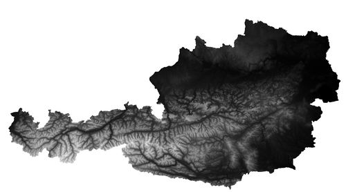
• A DEM raster file for Austria was obtained from the Government of Austria through Open Data Osterreich:

https://www.data.gv.at/katalog/dataset/b5de6975-417b-4320-afdb-eb2a9e2a1dbf Click on “zur Ressource” to obtain file.

• A geology shapefile of Austria was obtained from the Geological Survey of Austria (GBA):

https://www.geologie.ac.at/en/produkte-shop/geodaten-software/bersichtskarten/

• A soil shapefile of Austria Austrian Research Centre for Forests (BFW):

https://bfw.ac.at/rz/bfwcms2.web?dok=8548

• A landcover/land use raster file of Europe was obtained from the Copernicus Land Monitoring Service:

CLC_2018 Map https://land.copernicus.eu/pan-european/corine-land-cover Please note that you have to register to access the data, but registration is free.

Software Used

The exercises demonstrated are completed using the Quantum GIS 3.8.1 Zanzibar software interface. These are open source software materials which are freely accessible and available online. For new users it is suggested to use the standalone installer.

This is available by clicking this hyperlink. Click this!

Starting Map Project

The first step is to open QGIS and load all of the shapefiles and raster files into a new project. Vector files are added by selecting “Layer” on the top menu, then add “Add Layer”, and then “Add Vector Layer”. For the Raster Files, the procedure is similar, but “Add Raster Layer” is selected.

File Projections

The map projection used for this analysis was EPSG:31254-MGI/Austria GK West.

The initial file projections were as follows:

Vector Files:

• Austrian rail network shapefile: EPSG:4326 -WGS 84
• Political shapefile of Vorarlberg: EPSG:31254 MGI/Austria GK West
• Annual rainfall shapefile: 31254 MGI/Austria GK West
• Geology shapefile: 31287 – MGI Austria Lambert
• Soil shapefile: EPSG:3035 – ETR89

Raster Files:

• DEM Raster file:USER Generated CRS
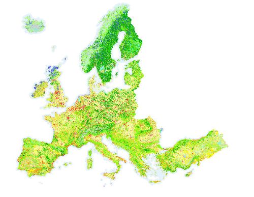
• Land cover/land use raster file: EPSG:3035 -ETRS89/LAEA Europe

Processing of the Vector Files

Reprojection of Vector Files

In order to prepare the vector files for use, they need have the correct projection: EPSG:31254 MGI/Austria GK West. The "Political" and "Annual rainfall" vectors have the correct projection, so the three remaining vector layers need to be re-projected: Austrian rail network (vector), Geology (Vector), and Soil(Vector).

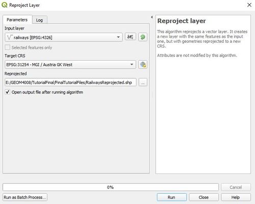
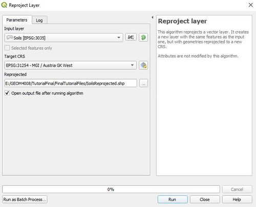
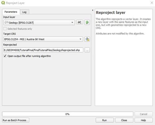
To re-project the three vector files, select “Vector” from the top menu, then “Data Management Tools” and “Reproject Layer”. On the “Reproject Layer” window, select the layer to be re-projected as the “Input Layer” and the “Target CRS” as EPSG:31254-MGI/Austria GK West. The “Reprojected” box is used to setup the file for the re-projected layer. Press the “…” button, select “Save to File’, select the project folder and a file name for the re-projected file. The image below shows the “Reproject Layer” window for the vector files that need to be re-projected:

Re-projection Window

Clipping Vector Files to Area of Interest

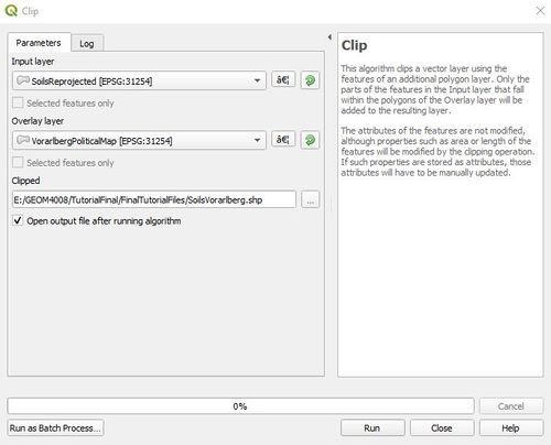
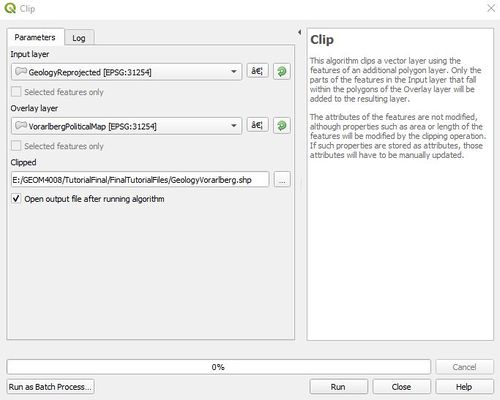
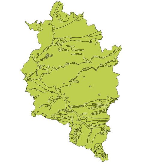
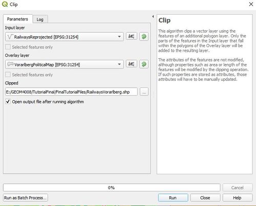
The next step is to clip the vector files to the area of interest, Vorarlberg Land. The Annual Rainfall shapefile is already for Vorarlberg, so the “Railways”, “Geology” and “Soils” shapefiles need to be clipped. To clip these vector files, select “Vector” from the top menu, then “Geoprocessing Tools”, then “Clip”. For the “Input layer”, select the file to be clipped (Railway Reprojected, SoilsReprojected or GeologyReprojected), then select the area of interest, Vorarlberg Political Map, as the “Overlay layer”. Under “Clipped”, select the “…” button, move to the folder where the project files are stored, and enter a name for the new layer under “File name” and press “Save”. This must be done for the three vectors to be clipped.

Clip Window

Railway lines in Vorarlberg Land

Soils in Vorarlberg Land

Geology in Vorarlberg Land

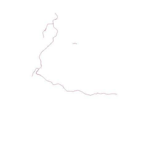
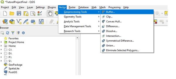
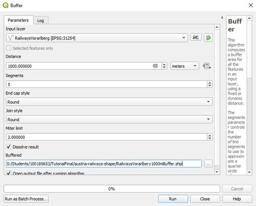
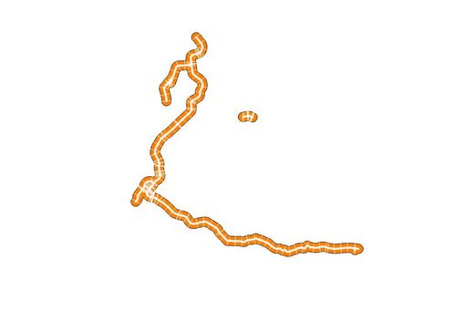
In order to find hazardous areas of concern around the rail lines, a buffer of 1000 metres was established on either side of the line. To do this, select "vector" from the top menu, then "Geoprocessing Tools" and then "Buffer".

In the Buffer window, select the RailwaysVorarlberg file as the "Input Layer", set 1000 meters under "Distance", and check off the "Dissolved result" checkbox. Lease all other parameters as default. Under "Buffered" select an appropriate filename for the buffered rail file and save in the appropriate directory by pressing the ... button and selecting 'Save to File..."

Railways lines in Vorarlberg with 1000 metre buffer on both sides.

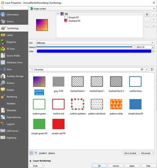
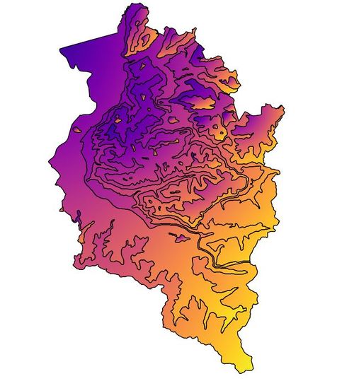
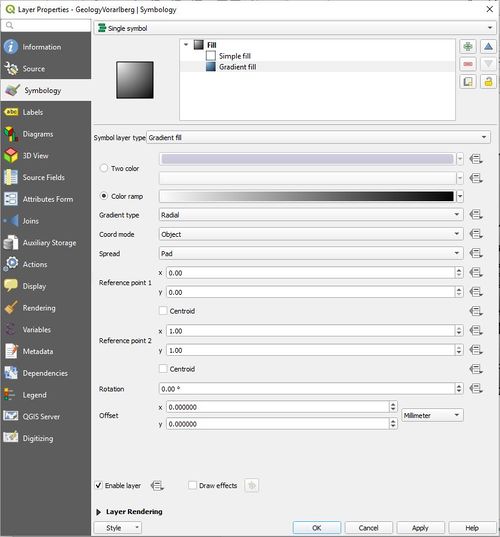
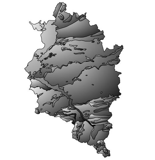
The next step is to change the colour scheme of two of the vector layers to bring out the contrasting data within the layer. The AnnualRainfallVorarlberg and GeologyVorarlberg layers will need to have their colours adjusted. To do this, highlight and right click on the layer in the “Layer Box” of the main project page, select “Properties”, and then “Symbology”. For the AnnualRainfallVorarlberg layer, select “gradient plasma” under the Favorites Box. Select “Apply” and then “Okay”. For the GeologyVorarlberg layer, complete the same procedure then select “Gradient Fill” in the top box and select “Grey” under the “color ramp”. Select “Apply” and then “Okay”.

Symbology Windows

Rainfall with new symbology.

Geology with new symbology

Selection of Potentially Hazardous Areas

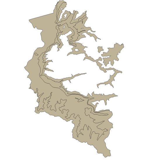
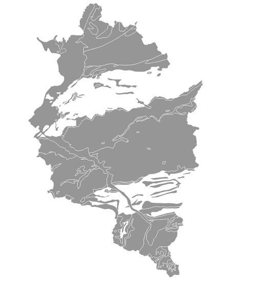
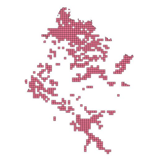
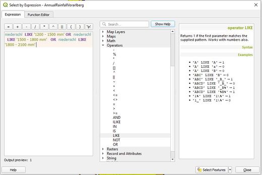
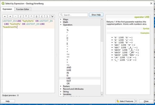
For each of the vector layers that define the characteristics of the Vorarlberg region, the attributes of interest that define hazardous areas must be selected. For “AnnualRainfallVorarlberg”, the rainfall is grouped in intervals between 1500 and 3000 mm , so the lowest three intervals were chosen: 1200-1500 mm, 1500-1800 mm and 1800-2100 mm. For GeologyVorarlberg layer, the rock types of interest were phylites, schists and sediments. For the SoilsVorarlberg layer, the soils of interest were clays (Lehm in German) and sand (Sand in German).

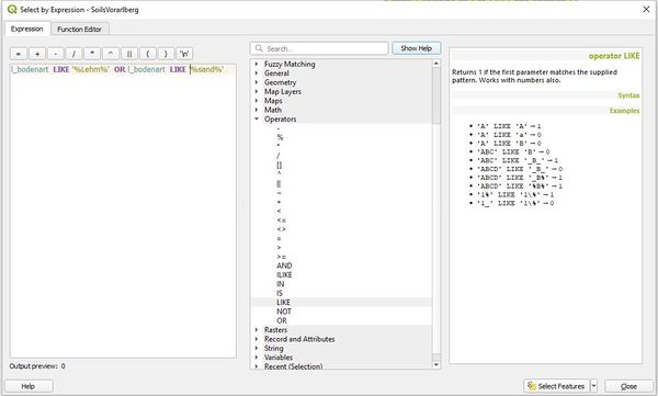
To select by attributes, the layer must be highlighted and right clicked in the main layer box and “Open Attribute Table” selected. Along the top of the attribute table are the headings for each column with the data in the columns below. From here, the “Select features using expression” button opens the “Select by expression” box (see below). The following expressions are entered in the left had expression box:

• AnnualRainfallVoralberg: niederschl LIKE ‘1200 – 1500 mm’ OR niederschl LIKE ‘1500 – 1800 mm’ OR niederschl LIKE ‘1800 – 2100 mm’
• GeologyVorarlberg: LEGTEXT_EN LIKE ‘%phylite%’ OR LEGTEXT_EN LIKE ‘%schist%’ OR LEGTEXT_EN LIKE ‘%sediment%’
• SoilsVorarlberg: l_bodenart LIKE ‘%Lehm%’ OR l_bodenart LIKE ‘%Sand%’

After entering the above equation in the “ Select by Expression” box, press “Select Features” at the bottom of the window and the selected features will be highlighted in the attribute table and map layer.

Select By Attributes Windows

Areas in Voarlberg with annual rainfall of 1200-1500 mm, 1500-1800 mm and 1800-2100 mm (yellow).

Areas in Vorarlberg with the following geological structures: phylite, schist or sediment(yellow).

Areas in Vorarlberg with clay or sandy soil (yellow).

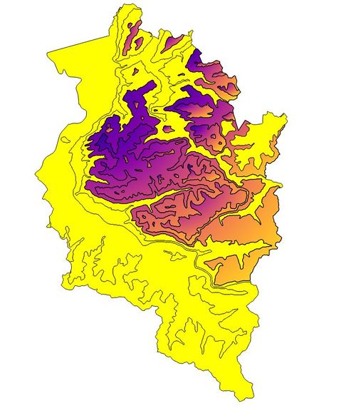
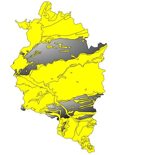
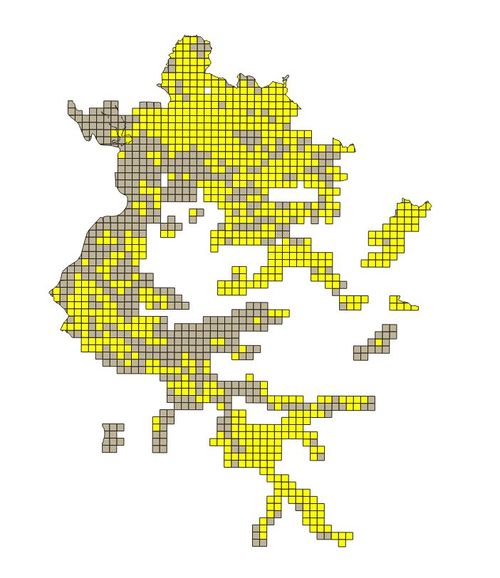
The next step is to save the selected attributes for each layer as a separate layer. Highlight the layer in the layer window, right click on it, select “export” and “Save selected features as”. In the “Save Vector Layer as” window, set the “Format” to ESRI Shapefile, use the … button to select the project directory and give the layer a file name, and check the “Save only selected features” box. The CRS should be set to EPSG:31254 MGI/Austria GK West.

The resulting layers

Rainfall Geology Soils

These three layers define areas of rainfall, geology and soils in Vorarlberg Land that could be potentially hazardous for linear infrastructure.

Processing of the Raster Files

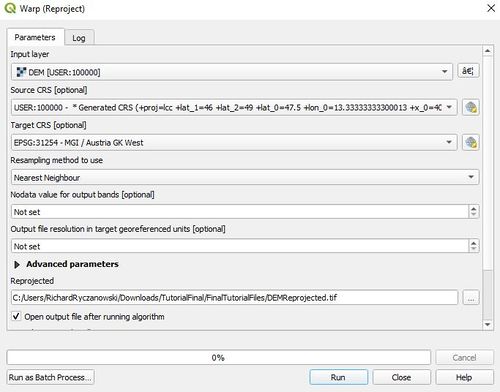
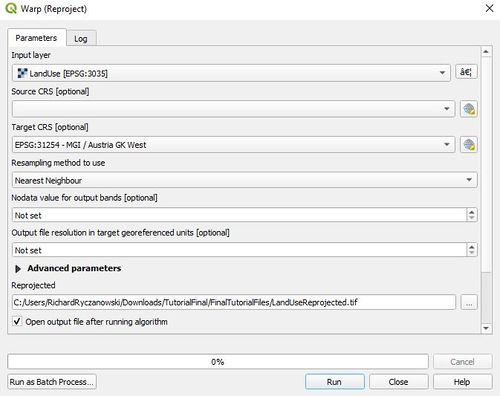
In order to use the raster files, they need to have the correct projection. Both the DEM and Land Use layers have to be reprojected to EPSG:31254-MGI/Austria GK West . In order to do this for each layer,"Raster" must be selected from the top menu, "Projections" from the drop down menu, and then "Warp (Reproject)" selected.

On the "Warp (Reproject)" window, select the original vector file as the "Input Layer", select EPSG:31254-MGI/Austria GK West as the "Target CRS" and define a new file for the output under "Reprojected". Leave all other parameters at the default settings. Pressing "Run" will start the reprojection process.

DEM

Land Use

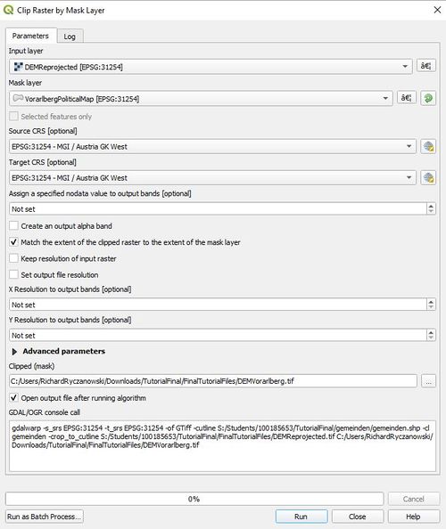
The raster layers must then be clipped to the extent of Vorarlberg Land. To accomplish this, "Raster" must be selected from the top menu, and "Extraction" from the drop down menu. For the Reprojected DEM file, "Clip Raster by Mask Layer" should the be selected. The "Input layer" is the DEMReprojected raster layer, and the "Mask Layer" is the Vorarlberg Political Map layer. Under "Advanced Parameters", a new file is defined for the clipped DEM layer under "Clipped (mask)"in an appropriate file directory.

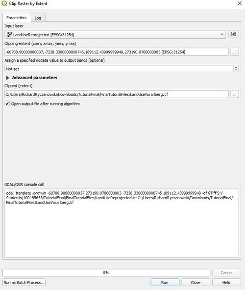
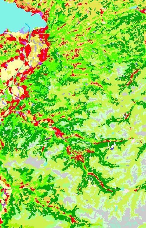
For the Land Use layer, "Raster" is selected from the top menu, then "Extraction" from the drop down menu, then "Clip Raster by Extent". On the Clip Raster by Extent window, the LandUseReprojected raster file is selected for "Input Layer" and the Vorarlbeg Political Map layer as the clipping extent. This is done by pressing the small...button at the end of the "Clipping extent (xmin,xmax,ymin, ymax) option, then selecting "Use Layer Extent" and then selecting VorarlbergPoliticalMap under "Use extent from". Under "Advanced Parameters" name a new file for the clipped land Use raster in an appropriate file directory.

DEM layer clipped to Vorarlberg area.

Land use layer clipped to the extent of Vorarlberg area.

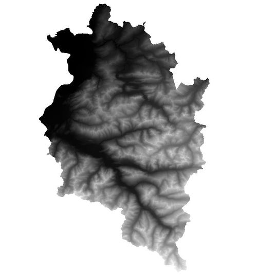
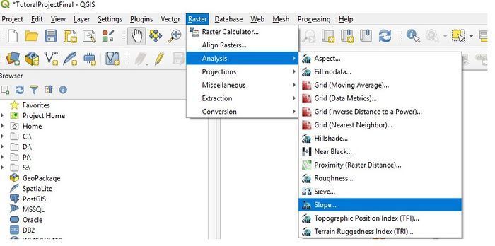
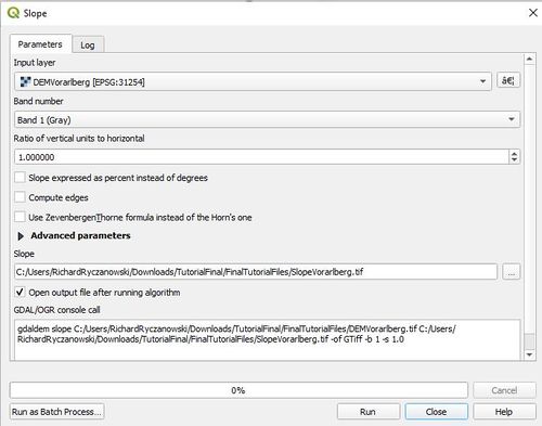
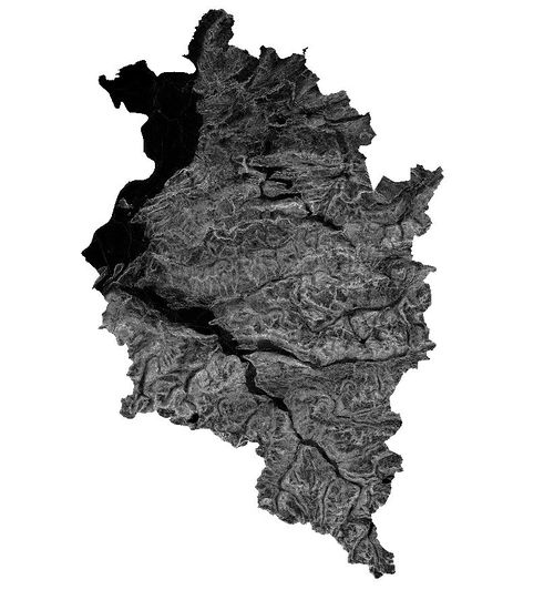
In order to find areas with hazardous slopes, the DEM layer will have to be converted into a slope layer. To do this, "Raster" is selected from the top menu, then "Analysis" from the drop down menu, then "Slope".

The DEM Vorarlberg layer is selected as the "Input layer" and under "Advance Parameters" and "Slope" specify a filename for the new slope layer in the appropriate project directory. Leave all other parameters at their default settings.

Slope layer for Vorarlberg area.

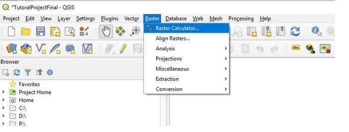
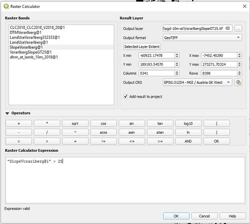
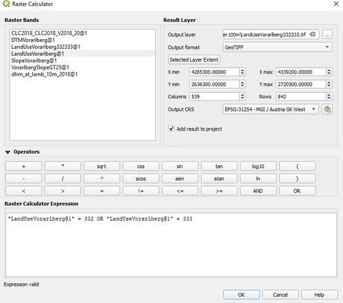
The next step is to identify those areas of slope and land use/cover that could be potentially hazardous. For the slope, those above 25 degrees are considered to be potentially hazardous. For land use/cover, potentially hazardous areas were bare rock (332) or sparsely vegetated (333). In order to select these area from the relevant raster layer, the raster calculator will be used. The Raster Calculator can be found under "Raster" on the main menu at the top.

On the raster Calculator window for the slope layer, Under "Raster Bands" select the Slope Vorarlberg layer. Under "Output Layer", select a name foe the new layer file for the selected areas in the appropriate directory. In the "Raster Calculator Expression" window, double click on the Slope Vorarlberg layer in the "Raster Bands" box and the operator buttons to enter the following equation:

"SlopeVorarlberg@1" > 25

Then press okay to start the selection operation.

For the Land Use layer, under "Raster Bands" in the "Raster Calculator" window select the Land Usee Vorarlberg layer. Under "Output Layer", select a name foe the new layer file for the selected areas in the appropriate directory. In the "Raster Calculator Expression" window, use double clicks on the Land Use Vorarlberg layer in the "Raster Bands" box and the operator buttons to enter the following equation:

"LandUseVorarlberg@1" = 332 OR "LandUseVorarlberg@1" = 333

Then press okay to start the selection operation.

Layer with slope greater than 25 degrees

Layer with bare rock or sparsely vegetated land use/cover.

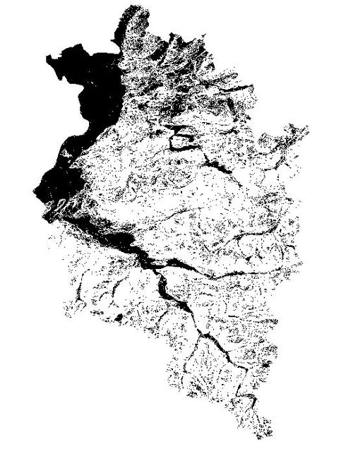
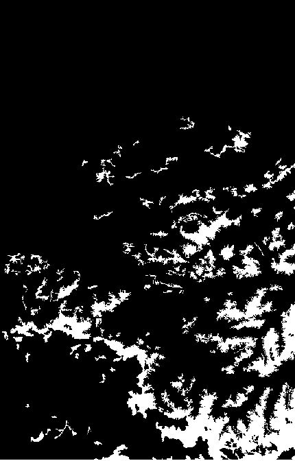
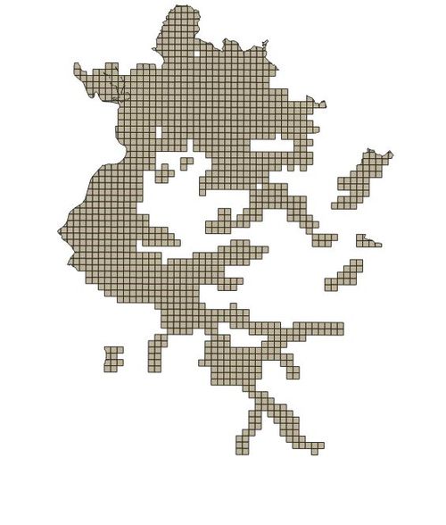
In both layers, the white areas are the ones that are potentially hazardous.

In order to further utilize the slope and land use raster layers, they must be converted into vector layers. To do this, the procedure is the same for both layers. Select "Raster" on the main menu at the top, then "Conversion" on the drop down menu, the "Polygonize (Raster to Vector)'. For the SlopeVorarlbergGT25 layer, select that file as the "Input layer". Then under "Vectorized", input a file name for the new Vorarlberg slopeGT25 layer in the appropriate project directory. Press Run to start the conversion process. the process is the same for the Land Use layer.

Vector layer for slope greater than 25 degrees.

Vector layer for bare rock and sparsely vegetated land use/cover.

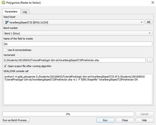
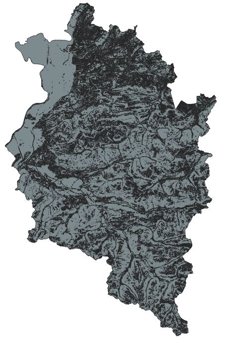
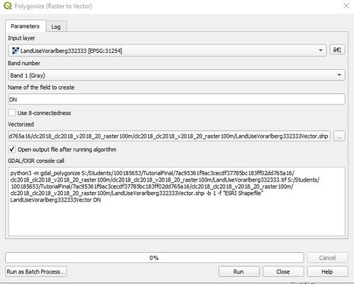
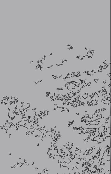
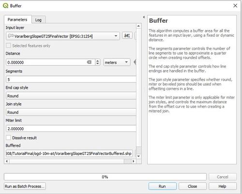
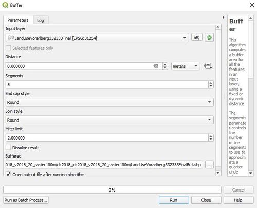
Unfortunately, the vectored layer output for both layers have an invalid geometry. To correct this problem, and make the layers usable for the rest of the analysis, a new vector layer must be created for each original layer with a buffer of zero. The procedure to do this for both layers is the same. Select ""Vector" from the main menu at the top, then "Geoprocessing tools", and then "Buffer". For the slope vector, select the SlopeVoralbergGT25FinalVector layer as the "Input layer" in the Buffer window, set the "Distance" to zero, and select a file name and directory for the new Slope GT25 Vector Buffered layer under "Buffered" and place in the appropriate directory. Leave all the other settings at their default. Press one to start the buffering process. The procedure is the same for the land use layer using the LandUsee 332333 vector file.

Intersecting the Layers

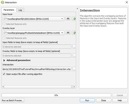
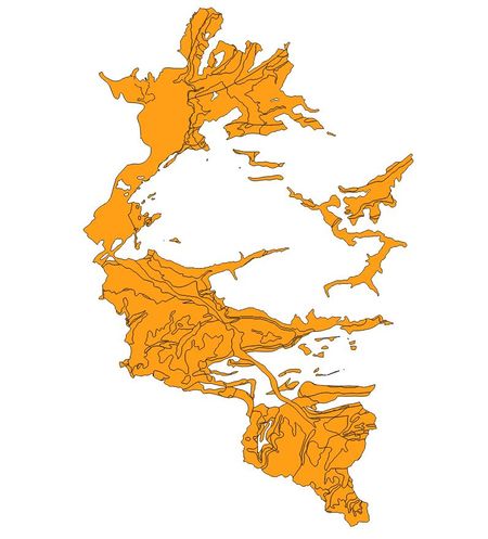
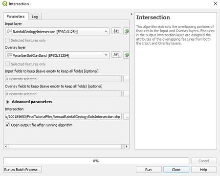
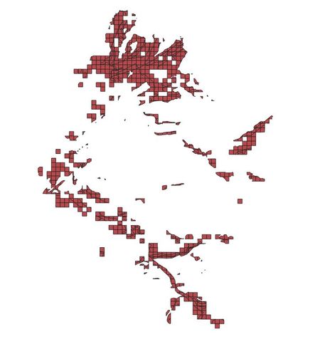
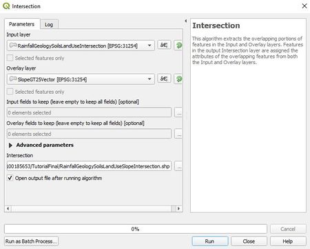
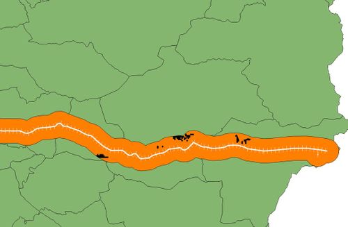
The final stage of this analysis is to intersect the five layers that have been used to define potentially hazardous areas (based on Annual Rainfall, Geology, Soils, Land Use and Slope)to determine the final area where the characteristics combine to make the area a combined hazardous area. To do this a series of intersection operations are performed:

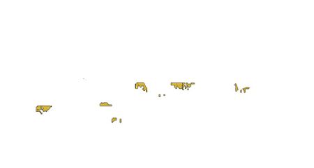
Annual Rainfall intersected with Geology to give AnnualRainfallGeologyIntersection AnnualRainfallGeology intersected with Soils to give AnnualRainfallGeologySoilsIntersection AnnualRainfallGeologySoils intersected with Land Use to give AnnualRainfallGeologySoilsLandUseIntersection AnnualRainfallGeologySoilsLandUse intersected with Slope to give AnnualRainfallGeologySoilsLandUseSlopeIntersection

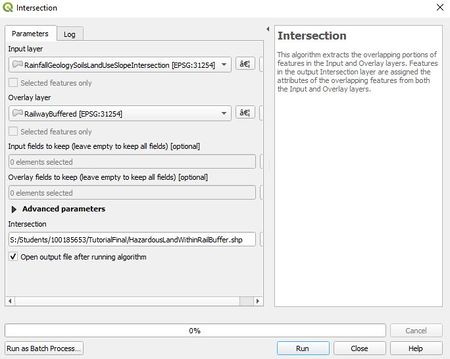
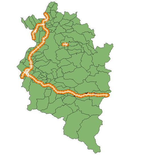
To give the final combined hazardous areas with the 1000 metre railway buffer:

AnnualRainfallGeologySoilsLandUseSlope intersects with Rail Buffer to give AnnualRainfallGeologySoilsLandUseSlopeRailBufferIntersection

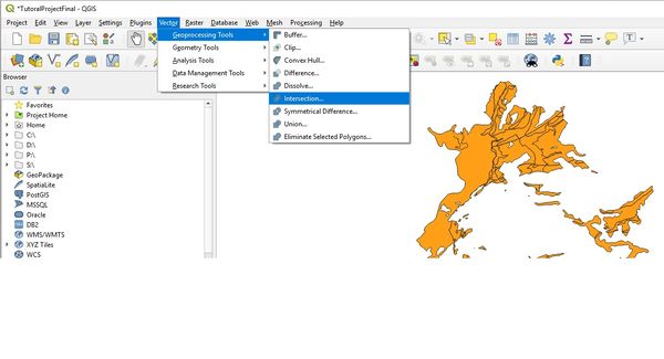
To create the intersection layers, select "Vector" from the top menu, then "Geoprocessing Tools", then "Intersection".

In the intersection window, under "Input Layer" select the first of the two layers that are to be intersected. In the"Overlay layer", select the second layer that is to be intersected. Under "Advanced Parameters, a new filename is entered for the new intersection file that is saved in the appropriate project directory. Leave all other options at their default settings. Pressing "Run" starts the intersection process. The Intersection Window for each of the five intersections are shown below with their output layers.

Rainfall and Geology Intersection Layer

Rainfall-Geology and Soils Intersection Layer

Rainfall-Geology-Soils and Land Use Intersection Layer

Rainfall-Geology-Soils-Landuse and Slope Intersection Layer

Rainfall-Geology-Soils-Landuse-Slope and Rail Buffer Intersection Layer

Final Maps

Here are the final maps showing the hazardous areas of concern for

Map of Vorarlberg showing hazardous areas along rail line

Zoomed in map of hazardous areas.

References

Laimer. H. 2017. Anthropogenically induced landslides – A challenge for railway infrastructure in mountainous regions. Engineering Geology. 222:92-101. Peruccacci, S., M. Brunetti, S. Gariano, M. Melillo, M. Rossi, and F. Guzzetti (2017). Rainfall thresholds for possible landslide occurrence in Italy. Geomorphology 290: 39-57. Rachoy C. and M. Scheikl (2006). Anthropogenic caused mass movements and their impact on railway lines in Austria. Pages 639 – 643 in H. Mauri and M. Mikos, editors. Disaster mitigation of debris flow, slope failures and landslides. Universal Academy Press, Tokyo, Japan.