Difference between revisions of "Unsupervised Landcover Classification In SNAP Using Sentinel 1 Imagery"
| Line 1: | Line 1: | ||
==[[Introduction]]== |
==[[Introduction]]== |
||
| − | ::Synthetic Aperture Radar, or SAR, is a method of RADAR imaging that propagates a microwave signal to |
+ | ::Synthetic Aperture Radar, or SAR, is a method of RADAR imaging that propagates a microwave signal to create an image over an area. The image is generates based on the type of backscatter that occurs when the signal hits a target. Unlike optical remote sensing, SAR is not affected by clouds or time of day; however, it can be adversely affected by heavy precipitation. |
| − | |||
| − | create an image over an area. The image is generates based on the type of backscatter that occurs when the signal hits a target. Unlike optical remote sensing, SAR is not affected by clouds or time of day; however, it can be adversely affected by heavy precipitation. |
||
This tutorial will use SAR data and image processing software to classify a RADAR image using an unsupervised classification method. |
This tutorial will use SAR data and image processing software to classify a RADAR image using an unsupervised classification method. |
||
Revision as of 18:30, 8 December 2019
Contents
Introduction
- Synthetic Aperture Radar, or SAR, is a method of RADAR imaging that propagates a microwave signal to create an image over an area. The image is generates based on the type of backscatter that occurs when the signal hits a target. Unlike optical remote sensing, SAR is not affected by clouds or time of day; however, it can be adversely affected by heavy precipitation.
This tutorial will use SAR data and image processing software to classify a RADAR image using an unsupervised classification method.
Unsupervised Classification
- Unsupervised classification aggregates spectral classes, or clusters, in a multiband image based on pixel value alone. This differs from supervised classification, where the user provides training data that the algorithm can use to assess the class to which a pixel belongs.
For unsupervised classification, the user instead tells the image classifier how many “clusters”, or classes, are desired, and what method to use.
In this tutorial, we will be using a K-Means classifier for the clustering algorithm.
- K-means is an algorithm that combines “observations” (in this case, pixels) into discrete
groups. It does this by creating nodes, which represent the center of a data cluster. This node is positioned so that the n distance between it and the nearest points is on average smaller than the distance between those points and the next node (Hunt-Walker & Ewing, 2014).
SNAP
- The Sentinel Application Platform, or SNAP, is an open source imagery analysis software provided by the European Space Agency. Along with the base tools, there are a number of other toolboxes available for more
complex analyses. It can be found here: http://step.esa.int/main/download/snap-download/previous-versions/
SNAP 7.0 has a bug in the software that effects a component of classification; therefore SNAP 6.0 should be used. The European Space Agency recommends SNAP be run on computers with at least 4GB of memory; however, for the classification, 16 GB would be preferred.
Data
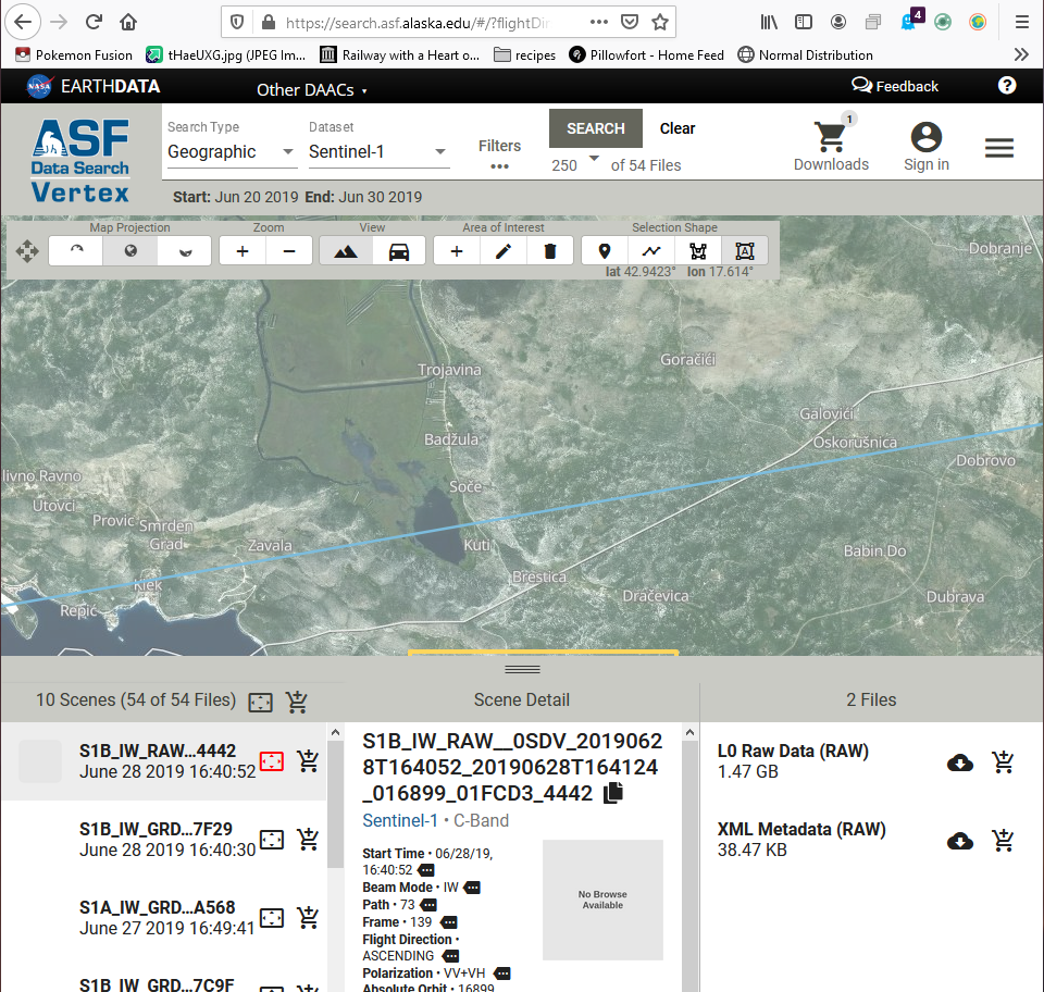
- To acquire data, you will need to register an account with the Alaska Data Search, found here: https://search.asf.alaska.edu/#/?flightDirs. To do so, go to the link and select “sign in” then “Register”. Follow
the instructions. This example uses the Bosnia and Herzegovinian and Croatian coastline. If desired, you can download several images and “stack” them. This process will be shown as well. Before selecting your images, you may wish to find out if it was raining in your AOI at your selected time. Precipitation has an adverse effect on radar.
Find the area of interest that you wish to classify.
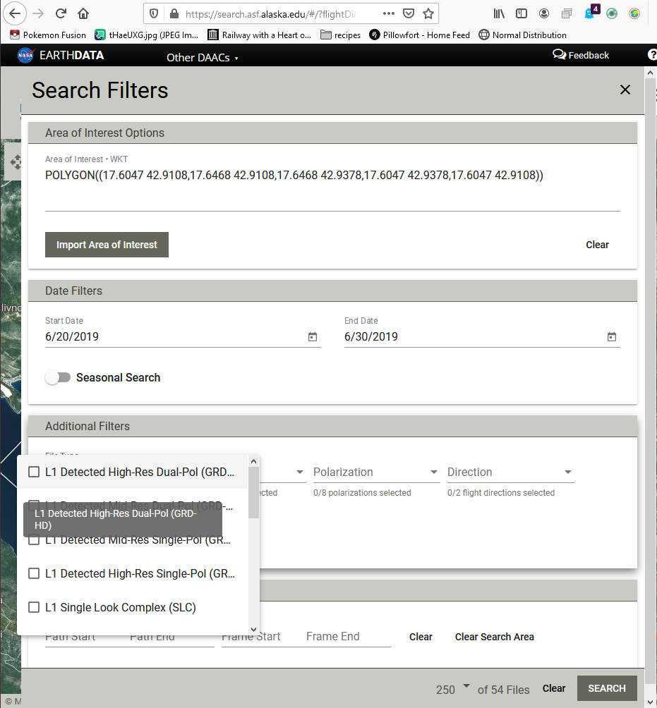
There is no need to use the exact image used in this tutorial, although the steps do require Sentinel 1 GRD format. GRD format can be input in the "Filters" window. If you do wish to use the image in the tutorial, parameters can be found below.
Example data Parameters
Search parameters:
Search type: Geographic
Dataset: Sentinel-1
Area of interest: POLYGON((17.6743 42.9283,18.3897 42.9283,18.3897 43.3711,17.6743 43.3711,17.6743 42.9283))
Start date:5/5/2019
End Date:6/13/2019
Under filters, select "L1 Detected High res Dual Pol(GRD)"
Frames: 140
Methods
- Set up your workspace by creating a file in the drive you wish to work in. Save your images to this file.
- Open SNAP.
Import your data into SNAP using the “import Product” button, and navigate to your working folder.
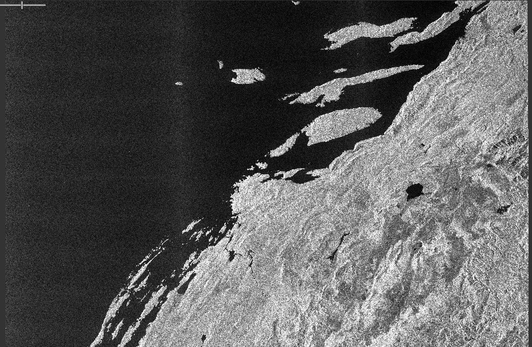
To get a feel for what your data looks like, double click on it to expand, then the “Bands” folder. Double click any band, and an image will appear of that band's backscatter imagery.
The band you open should look somewhat similar to the image above.
Preprocessing
1. Subsetting
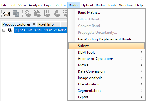
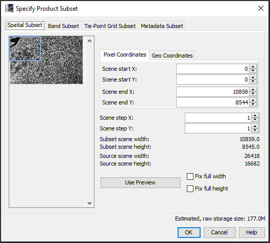
- The next step will be to subset your image. Because of the time it takes to do unsupervised classification, you may wish to make a very small image.
Navigate to Raster->subset
It is easiest to make a subset by dragging each side of the blue box on the left to the size you want, then selecting the middle and moving it to an area of the thumbnail. Once you are satisfied, select the “Okay” button.
If you wish to incorporate other images, you will want to copy the Scene Start and End values, or the geocoordinates, in order for your data to stack properly.
Then, right click the subset and select "save product as" and save to your working directory. Repeat on all your chosen images.
Then, it is time to preprocess your image. Preprocessing is necessary because a raw SAR image can contain missing or incorrect information.
Ensure you are writing to the working directory for all preprocessing and classification steps, and performing each step on each subsequent image.
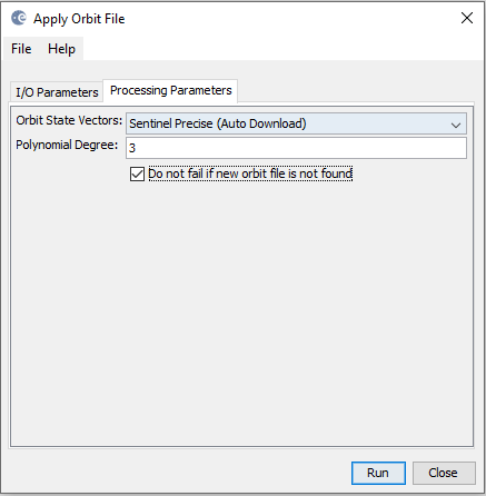
Application of Orbit File
Over time, satellites can drift, and their orbit must be corrected. This can effect the recorded location of the image. To account for this orbital drift, SNAP can download current satellite information. To apply an orbit file, navigate to Radar->Apply Orbit File. The default of Sentinel Precise does not need to be changed, but "Do not fail if new orbit file is not found" should be toggled. .
Backscatter Conversion
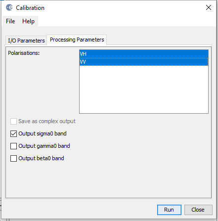
Radiometric calibration normalizes variations in RADAR system responses.
Navigate to Radar->Radiometric->Calibrate.
Select both bands, and leave "sigma" toggled.
Run.
Speckle Filter
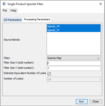
Speckle is "noise" in a SAR image. Filtering suppresses noise effects and makes an image clearer. Type and size of filter depends on application. We will use a 7x7 Gamma Map, as this is what Agriculture and Agri- Food Canada uses for image classification.
Radar->Speckle Filtering-> Single Product Speckle Filter
Select all bands.
find "Gamma Map" in the dropdown menu.
Type 7 in both the X and Y fields.
Run.
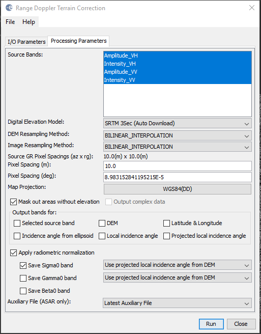
Geometric Correction
Terrain correction corrects for satellite tilt so that the geometric representation of the image is approximate to real-world topography.
Radar->Terrain Correction-> Range-Doppler Terrain Correction
Select all bands.
Leave default values.
Toggle "Apply radiometric normalization".
run.
If you only intend to run the classification on one image, skip the next step. If not, continue on to Coregistration.
Coregistration
If you intend to run the classification on multiple images, you will need to "stack" them. To do this, navigate to Radar->Coregistration->Coregistration. Add all your subset and preprocessed images by selecting either "add" (symbolized in 6.0 as a + sign) or "add opened" (symbolized as a + with a square background). In the CreateStack tab, select "Bilinear Interpolation" for the resampling type, and select "find Optimal Master". Cross-Correlation and Warp tabs can remain default values. In the "Write" tab, save to your working directory. Run.
Classification
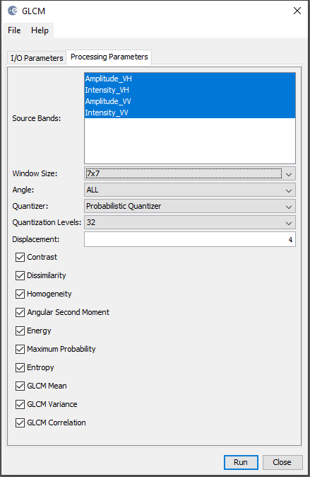
Due to the nature of SAR data, texture is critical to accurate classification Therefore, we will use the GLCM texture analysis to generate texture bands. This can be a time consuming process, depending on the size of your image.
To apply the GLCM, navigate to Raster->Image Analysis->Texture Analysis-> Grey Level Co-occurrence Matrix
In processing parameters, ensure all your bands are selected, and use a 7x7 window. all other variables can remain as default.
Run.
Once the GLCM is complete, you can apply the classification.
Classification Raster->Classification->Unsupervised Classification-> K-Means
Select the number of clusters you wish your image to have; for this example, there was three clusters of interest, but depending on your AOI there can be less or more. Both number of iterations and random seed can be left as the default. Select all the source bands you wish the classifier to use. Run.
Note that this can be quite time consuming; however, if it has no progress after an hour or so, you may need to subset your image smaller, or reduce the amount of bands used for classification.
