Wind turbine location suitability

Introduction

With the growing expansion of the city Ottawa energy capacity requirements become an integral issue. Currently the Energy Ottawa Company supplies a majority of its energy to the city through what is known as the ‘run-of-the-river’ generating system. This is a series of small scale hydroelectric dam facilities spread out across the regions watershed (Energy Ottawa, 2010).

This method of energy generation is considered a green means of producing energy, as it does not typically involve emitting pollution into the atmosphere compared to coal, petroleum, or natural gas. What is often overlooked is the negative affects that hydroelectric dams pose to the health of watershed, impacting many aspects of both the natural and social environment. These adverse affects have caused the number of hydroelectric dams being built to be drastically reduced in Canada (Natural Resources Canada [NRC], 2009).

This has led many municipal and provincial governments to seek alternative green energy production techniques. As such wind energy has come to the forefront of this search. Wind energy is however not without its negative implications as well. Recent studies have been produced in which attribute the construction of wind farms as causing degradation the environment in sensitive areas, as well as possibly having negative implications to human health with prolonged exposure in close proximity to wind turbines. To mediate these concerns the provincial government of Ontario has released various restrictions, limiting areas in which the construction of wind farms is permitted.

Objective

The objective of this tutorial is to demonstrate a technique which identifies spatial regions deemed as potentially suitable locations for the development of wind energy production. This will display means for consideration of the restrictions imposed by the provincial government to evaluate the purposed region. The desire of this particular case is to identify suitable locations for wind energy production in Ward 21 of the Ottawa, Ontario region.

Restrictions

The Provincial Government of Ontario has provided the following restrictions in relation to the spatial placement of wind energy turbines for use of commercial applications:

• 135m from all existing public roadways

• 135m from all existing railway lines

• 1000m from all existing transmission lines

*These restrictions are relative to the turbine specifications of the Vestas V90, 3 megawatt model

These restrictions were provided by:

• Renewable Energy Approvals
• Technical Bulletin Six: Required Setbacks for Wind Turbines
• Drafted by the Environmental Registry March 1, 2010

Methods

The following will thoroughly demonstrate the techniques involved in this approach for identifying suitable wind energy production sites in the Ottawa city area. This example looks to specifically examine Ward 21, Rideau-Goulbourn.

Data Used

The first step is to gather all necessary data appropriate for the purpose of this exercise. This example uses vector shapefiles which include:

• Ottawa area boundary
• Ottawa city wards boundary
• Transmission lines
• Railways
• Federal Roads
• Provincial Roads
• Regional Roads

This data can be gathered at http://data.ottawa.ca/ or at http://geo1.scholarsportal.info

Software Used

The exercises demonstrated are completed using the Quantum GIS software interface. These are open source software materials which are freely accessible and available online. For new users it is suggested to use the standalone installer.

This is available by clicking this hyperlink. Click this!

This is based on the OSGeo4W packages and includes the newest version of qGIS (2.18.13) as well as the GRASS toolset.

Starting Map Project

Before beginning it is recommended to always rename all shapefiles you create in the Layer Panel, to make sure you do not get confused with your files.

1. Begin by opening the Quantum GIS software. Select ‘Layer’ from the drop down menu and open the ‘add vector layer’ function or click the ‘add vector layer’ icon on the toolbar. Ensure source type is set to ‘file’. Locate vector dataset by selecting ‘browse’ and open a shapfile which will be used for the project. Click ‘open’ and the shapefile will be added and displayed. Repeat this process until all shapefiles intended for use have added.
2. Once all vectors have been added, you should set the coordinate reference system (CRS). Select 'Layer' go to 'Set CRS of Layer(s)' and select which CRS you want.
   1. The recommended CRS is MTM 9, and when this is selected from the drop down menu, click OK and the layers you added are set with that CRS.
3. Next the vector files must be clipped to fit within the extent of the Ottawa area. If all your data fits within the boundaries of Ottawa, skip this step.
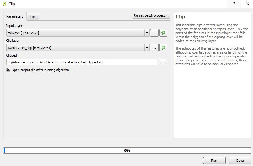
   1. Select the 'Vector' tab and go to the 'Geoprocessing' menu, and select the clip tool.
   2. In the 'Input layer' section select the layers that need to be clipped down. Do this individually for each layer that needs to be clipped.
   3. In the 'Clip layer' section select the layer that will act as your extent, the Ottawa area. It should be the wards layer.
   4. The following section is for deciding your output. Click the 3-dot button and and select save to file. Name your new file with details (example: rail_clipped), and save click save in that new window.
   5. Make sure the box under the output section is checked to allow the program to automatically add it to your working layers.
4. If the clipping tool has a blank output this is the solution to that problem. Skip if the Clipping worked.
   1. If the you get a warning message that the CRS do not align and will cause problems, the solution is to enable the 'on the fly' setting and reproject a CRS of the problem layer.
   2. Click the CRS button on the bottom toolbar of the program, beside the speech bubble. At the top of that popup, you want to enable the 'On the fly' transformation, if it is not enabled already.
   3. From here, select the layer in the Layers Panel that is not aligning with your desired CRS, and right click it. From this menu select the 'save as' option and create the same shapefile with a new name, and with the CRS of the project. This creates the shapefile again, but this time with the CRS aligning with the project, and allowing you to work with the layers using geoprocessing tools.

Narrowing Results to a Specific Delineation Area

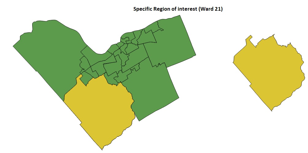
This section focuses on narrowing the view to a specific area of interest. In this case the area of interest is Ward 21, Rideau-Goulbourn. This is a largely rural/agricultural ward of the city making it a prospective optimal area for the production of wind energy. This process will involve the exporting of the specified area as a new shapefile.

1. The following steps demonstrate the exportation of a specific area of interest as a new shapefile:
   1. Right click the wards layer in the layer panel, and select the attribute table.
   2. Next, select the ward you want to create a new shapefile out of, this time being ward 21.
   3. Close the attribute table, and select the edit tab from the top, and select 'Copy features' in the menu.
   4. Open the same menu and select 'Paste As' this time, and select 'New vector layer'.
   5. In this popup name your new shapefile (example: ward21) and make sure the CRS is the same, and click 'OK' to create the subject area shapefile.
   6. Add the newly created shapefile to the map project if not already present.
2. With the new ward extent shapefile, you want to trim the extra data down to fit within it.
   1. It is similar to the clipping tool, but this time select the 'Intersection' tool.
   2. Input the data you want to cut down, the polyline data, and show them instead of the full extent shapefiles.

Visualization of Restrictions using a Buffer

This portion will demonstrate how to imply a buffer region to each of the vector polyline layers representing limitations imposed by the spatial restrictions set by the Provincial Government of Ontario.

1. Open the 'Vector' tab and go to the 'Geoprocessing' menu, and select the 'fixed distance buffer' tool
2. To create the railway buffer, select the Railway Lines layer under the 'Input layer' field
   1. Set the 'Distance' field to 135 (this number represents the 135m restriction applied to Railways)
   2. Leave 'Segment' as the default 5, as changing this does not have a significant impact on the end result.
   3. Then set the name for output vector map (example: RailwayBuffer)
   4. Make sure the dissolve box is checked, which makes the buffer a continuous shape, instead of separate entities.
   5. Click Run, and wait for the output to successfully finish (this may take an extended period of time depending on the size of the input vector layer
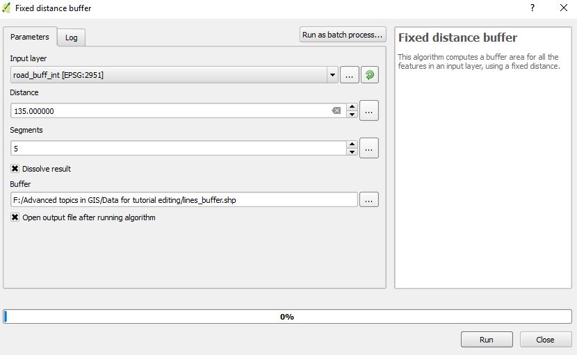
3. Complete this process for Road Layers again setting the 'Distance' to 135 as the restriction for roads is the same as railways.
4. When completing this process for the Transmission Lines layer make sure to change the 'Distance' parameter to 1000 to meet the 1000m restriction imposed on this infrastructure.

Representation of the Resulting Layers:

Creation of Total Suitable Areas Using an Overlay

This section will demonstrate the use of vector overlay techniques in order to visualize total suitable areas free of spatial restrictions.

1. Select the 'Vector' tab, select 'Geoprocessing tools' and select 'Union' as the last part of the menu.
   1. Under the 'input layer' field choose the Railway Buffer layer.
   2. Under the 'input layer 2' field choose the Transmission Lines Buffer layer.
   3. Under the 'Union' field provide an output name (example: RailHydroOverlay)
   4. Click run, and wait for the output to successfully finish.
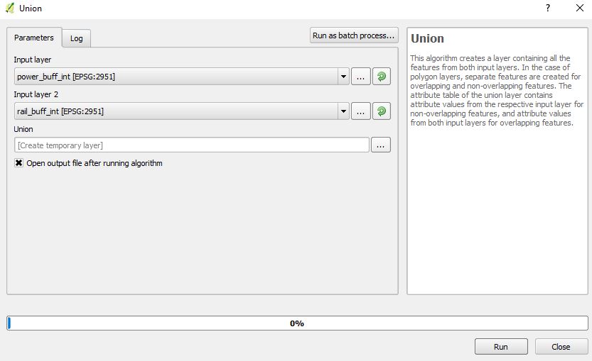
2. Return to the 'Union' tool.
   1. Under the 'Input layer' field choose the Union layer just created (example: RailHydroOverlay).
   2. Under the 'Input layer 2' field choose the Roads Buffer layer.
   3. Under the 'Union' field provide an output name (example: MergedBuffers)
   4. Click run, and wait for the output to successfully finish.
3. Return to the 'Geoprocessing tools' tab and select the tool 'Dissolve'. This will clean up the merged layers.
   1. Select the shapefile you just created as the final merge, and check the box 'Dissolve All'.

This process results in the overlay of all three buffer restriction layers providing a total suitability layer which considers all restrictions.

Representation of the Resulting Layer:

Identifying Largest Suitable Area

The Largest suitable area can be identified using the 'measurement tool' located on the toolbar. However, this would take a lot of time to outline each shape, so I will show you a way to calculate each area.

1. The first step is to go 'Vector'>'Geoprocessing'> 'Difference'.
   1. Select the extent area as the input and the merged buffers as the difference.
2. You now can see each individual shape away from the buffers, which allows us to calculate the area of each shape.
   1. First we must separate them in the attribute table, and to do this we must create another shapefile. To do this go 'Vector'>'Geometry'> 'Multiparts to Singleparts'.
   2. Select the created shapefile from the 'Difference' tool and create a new shapefile of separated features.
3. Now turn on editing of this new shapefile, and open the attribute table to reveal the large number of features present in this shapefile.
   1. You can turn on editing by right-clicking the layer in the Layer Panel and selecting the 'Toggle Editing' option.
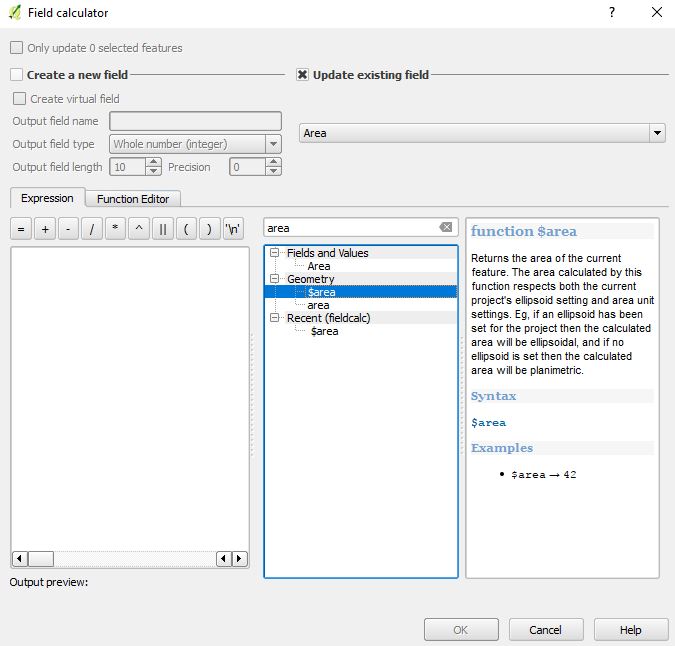
   2. Once in the attribute table create a new field. You will want to name the field "area" and select 'Decimal Number'. Precision and Length can be left default.
   3. Now open the 'Field Calculator' and select 'Update existing field' and select the field you created.
   4. In the search bar below, type in "area" and select the option named "$area"
   5. press 'OK' and all shapes will have an updated area field in meters squared. Sort the new field to find the largest in terms of area.
4. Once the largest suitable area has been identified, create a new vector polygon to represent this area. This can be done with the same process as creating a smaller extent from earlier.

Representation of the Resulting Layer:

The resulting layer provides the largest suitable area for the specific region of interest with the consideration of all implied restrictions. By combining all the final layers together, you would get a map that shows the most suitable location based on area for wind turbines, along with the provincial restrictions set in place. This process is doable for any of the wards in the Ottawa region, and could be used to select different areas with different restrictions, all depending on the data present.

References

• Energy Ottawa. (2010). "Green Power". Accessed online: http://www.energyottawa.com/forms/index.cfm?dsp=template&act=view3&template_id=46&lang=e
• Natural Resources Canada. (2009). “Hydroelectric Generation”. The Atlas of Canada. Accessed online:http://atlas.nrcan.gc.ca/auth/english/maps/freshwater/consumption/hydroelectric/1