Automating Vector and Raster Workflows using the Graphical Modeler in QGIS

Disclaimer

Please note that this tutorial was created as a term project for the Carleton University class GEOM4008 - Advanced Topics in Geographic Information Systems. The tools used below are just some of many that can be found within QGIS and outputs may heavily vary depending on the inputs. The results should not be used as conclusive findings for others work.

Introduction

The objective of this tutorial is to provide an in-depth walk through of automating two workflows in the QGIS Graphical Modeler. The first is a simple workflow using sample vector data that covers geoprocessing tools such as buffer, clip and merge. It will also demonstrate how to perform a field calculation within a model. The second workflow is more complicated and works with a sample Digital Elevation Model (DEM). The workflow covers the various steps required to determine the watershed basins within an area of interest. The different algorithms covered in this tutorial are: fill sinks, catchment area, channel network, watershed basins and vectorising grid classes. These algorithms are native to SAGA GIS, but through QGIS's advanced interface processing toolbox, they, as well as GRASS GIS algorithms, are accessible. This tutorial provides a highly explanatory and easy walk through for individuals with varying levels of GIS knowledge. The purpose is to aid those looking for a quicker, more efficient way of performing long workflows without the use of expensive GIS software.

Software

As mentioned above, the software that will be used for this tutorial is Quantum GIS, otherwise known as QGIS. It was chosen for two reasons; first, it is one of the most powerful GIS FOSS (Free and Open-Source Software) packages, with a very user friendly interface; second, it has a very intuitive Graphical Modeler that has access to many different algorithms from GDAL, GRASS, ORFEO Toolbox, QGIS and SAGA. Along with being very powerful and free, it is also available for all common computer platforms (Windows, Mac OS X, Linux, BSD, and Android).

In order to follow along with this tutorial, the first step is to download QGIS:

http://www.qgis.org/en/site/forusers/index.html

From this website, you will find a link to download the software to the appropriate platform and documentation for getting started.

NOTE: This tutorial was completed in QGIS 2.8.0 therefore depending on your version, somethings may have changed.

Data

The data for these tutorial originates from two websites. The first set of data required for the vector workflow tutorial is available from the City of Ottawa Open Data website. The data sets required are:

Roads - http://data.ottawa.ca/dataset/roads

Proposed Roads - http://data.ottawa.ca/dataset/roads-proposed

Water bodies - http://data.ottawa.ca/dataset/water

NOTE: Make sure to select the download link associated with the SHP format.

For the raster workflow tutorial, the only required data is a DEM of whatever area you are interested in. For this tutorial, the DEM will be accessed through Scholars GeoPortal which houses huge amounts of geospatial data that are freely available to those studying within one of the 21 schools that fall within the Ontario Council of University Libraries (OCUL). The DEM chosen from Scholars Geoportal comes from the retired Ministry of Natural Resources Provincial Digital Elevation Model Dataset - Version 2.0.0. The DEM covers a portion of Eastern Algonquin Park, located around the Barron Canyon (20km x 13km), and has a cell resolution of 10m.

Tutorial for Automating a Vector Workflow

With QGIS open, the first thing to do is to add the vector data.

Adding Vector Data

There are 2 methods for adding vector data into QGIS. The first method is to simply just drag-and-drop the vector layer file you would like to add. The second method involves using the menus and is highlighted below.

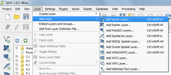
• Along the top toolbar, select Layer --> Add Layer --> Add Vector Layer

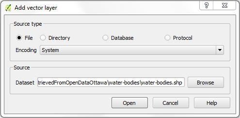
• After selecting Add Vector Layer, a dialog box will pop-up and this is where you will browse for the Vector Layer you are looking to add

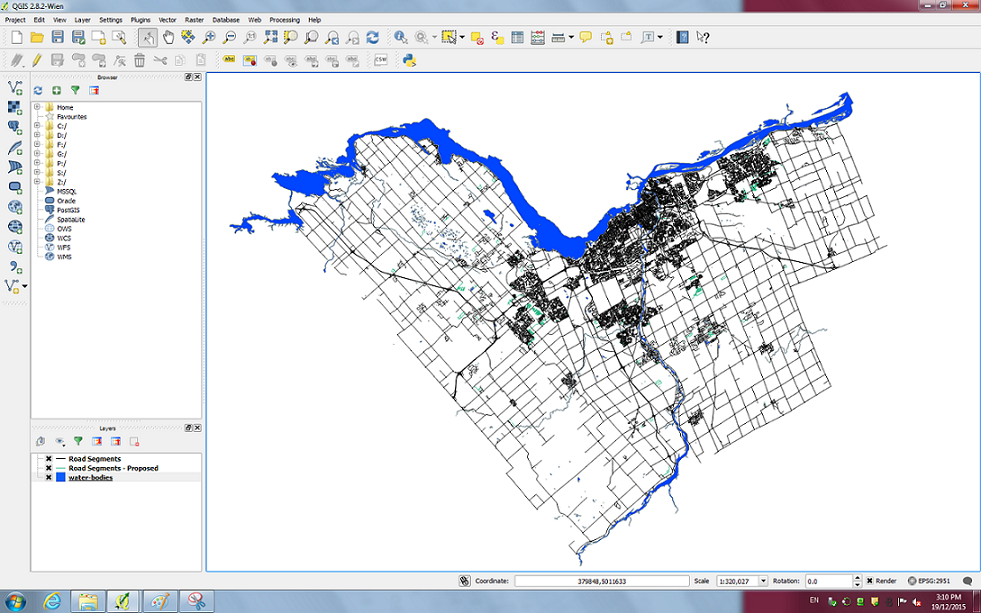
• For the tutorial, this will be done 3 times in order to add our roads, proposed roads and our water bodies. Below you will find what QGIS looks like with all 3 layers added.

Opening the Graphical Modeler

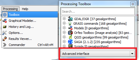
• Before we begin creating the model we need to change the processing toolbox interface from Simple --> Advanced. This option can be located at the bottom of the processing toolbox.

• Without changing it to advanced, inside the Graphical Modeler, you would only have the ability to use the simple interface algorithms

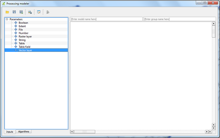
• To open the Graphical Modeler, in the top toolbar go to Processing --> Graphical Modeler. The window should look like the one below.

Creating the Input Parameters

• In the figure above, you'll notice many types of input parameters with "+" signs next to them. In order to add in a vector layer parameter, double click on that option.

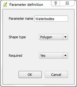
• In the dialog box that pops up, give the layer a name unique name, change the shape type to match the data type (point, line or polygon) and set required to Yes.

• Do this 2 more times for the other 2 vector layers.

• After adding all 3, the Graphical Modeler window will look like this:

Creating the Model

Buffer

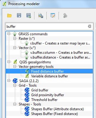
• Creating the model is actually relatively simple. Search for the desired tool, then double click on it and set the parameters. Here, we'll use the fixed distance buffer tool:

.

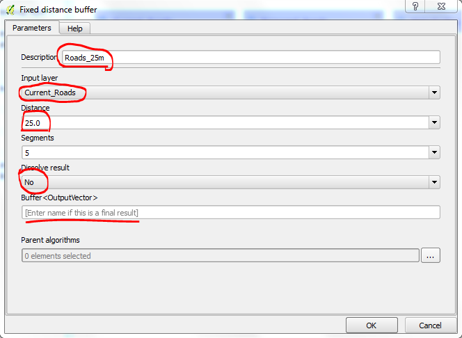
• Make sure to set a description to differentiate it from the others, as well, set the proper input layer.

• Specifically for the Buffer above, I decided on a 25.0m buffer of the roads and unless you have plenty of time, set dissolve to NO.

• You'll notice no output vector was specified and that is because it is not required until the last tool in the model or whenever an output is desired.

• Do this for both of the Roads files with the same parameters other than the input layer.

Merge

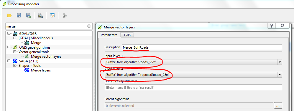
• With both of the road layers buffered, we will now merge them into one road layer (you can also merge first and then buffer, whatever tickles your fancy). Refer to the image below for which tool to use and how to set the parameters.

Clip

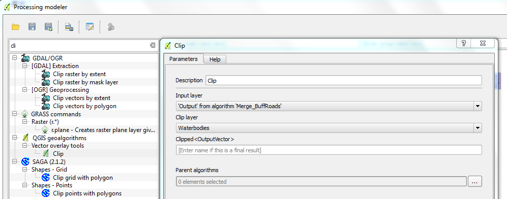
• Now that the road buffers have been merged, we will use the QGIS vector overlay clip tool too determine where there is overlap between the road buffers and the water bodies.

• The clip can be performed either way (i.e. the input layer and the clip layer can be switched if you please).

Field Calculator

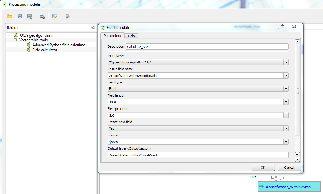
• In order for us to determine the amount of area where a 25m road buffer would overlap the water bodies, we will perform a field calculation. Refer to the image below to the input layer, field type, length and precision and for the formula

IMPORTANT NOTE:

• As this is the last step in the model, we now are required to specify an output layer, so do not forget to do that (this can be seen as the blue rectangle that appears under the Field Calculator dialog box.

Final Look

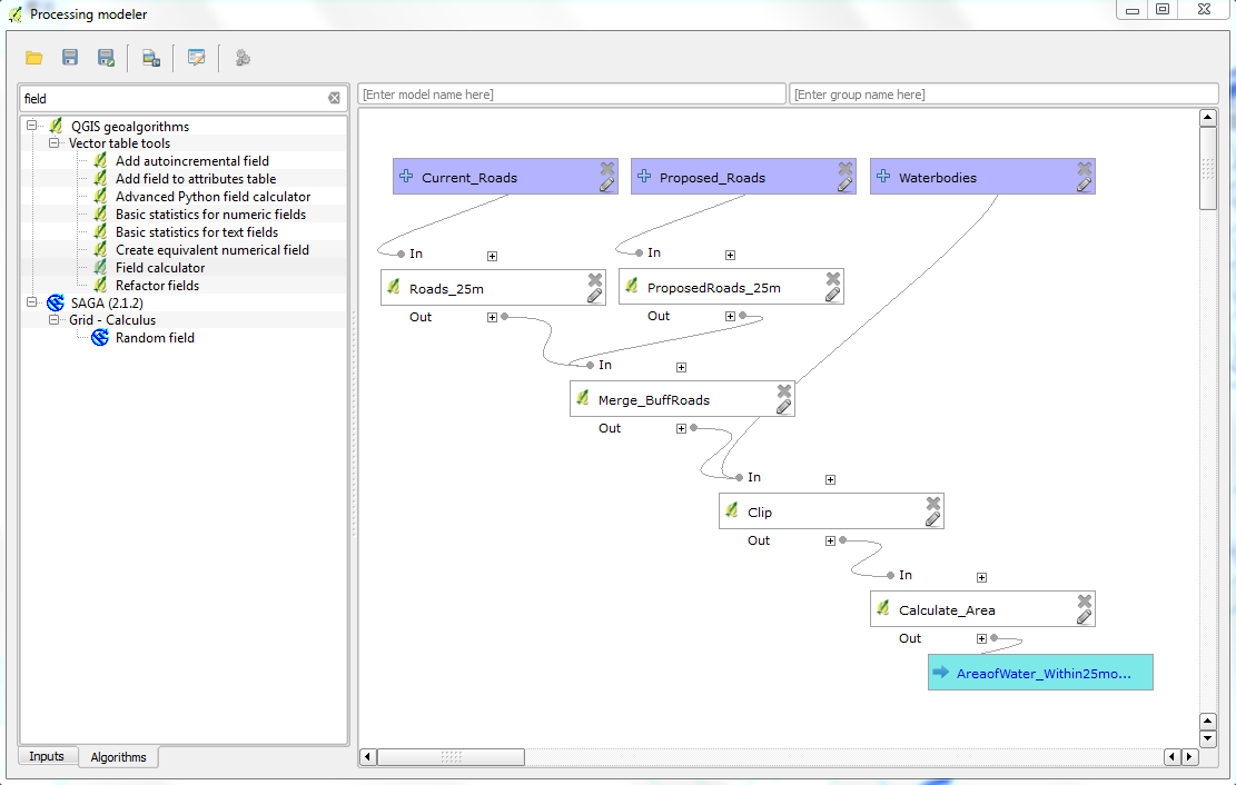
• With the model now built, I recommend taking this time to go back through the tools (selecting the pencil in the bottom right hand corner of each processes) to make sure all the inputs and parameters are set correctly.
• The model should look a little something like the one found below.

Save & Run

• With the model built and double checked we can go ahead and save the model. Enter a model name and a group name, then select the red-underlined button third from the left to save the model in an appropriate location. Lastly, select the circled button in order to run the model.

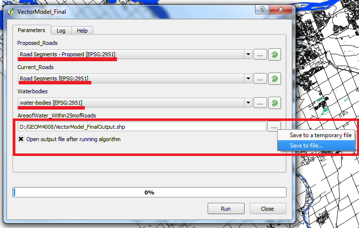
• Once the run button is clicked, you will be asked the set the layers to match the input vector parametres.

• Lastly, save an output and make sure the box is checked to allow for the output file to open once the model is finished running.

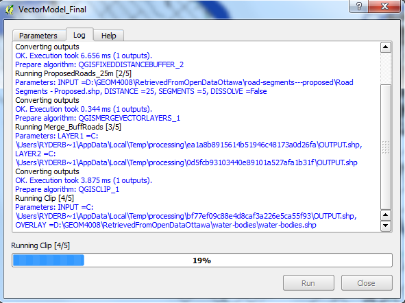
• While the model is running, you will notice which step the model is on (ex: 4/5)

Output

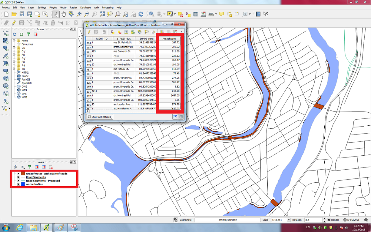
• With the model finished, you will notice an added layer in the table of contents.

• As well, we can check the attribute table to make sure the field calculator process ran and as you can see below, it worked properly.

Tutorial for Automating a Raster Workflow

Since the instructions above have already provided very extensive details, in this section we will primarily stick to the larger steps, assuming you have already mastered the simpler tasks.

Adding the DEM

• Adding a DEM can be done using the same two methods as mentioned in the vector tutorial (Drag and Drop or through the menus).
• To add a DEM through the menus, go to Layer --> Add Layer --> Add Raster Layer then find the DEM through the windows explorer dialog box.
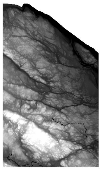
• Below is the sample DEM for this tutorial (black = low elevation, white = high elevation)

Creating a Mask and Clipping

• In order to allow for a faster workflow, we will clip the DEM using a mask (i.e. an area of interest)
• To do so, go to Layer --> Create Layer --> New Shapefile Layer and double click
• Set the type to Polygon and set the CRS that matches the EPSG code found at the bottom right hand side of the QGIS window.
• Save the new layer to an appropriate location.

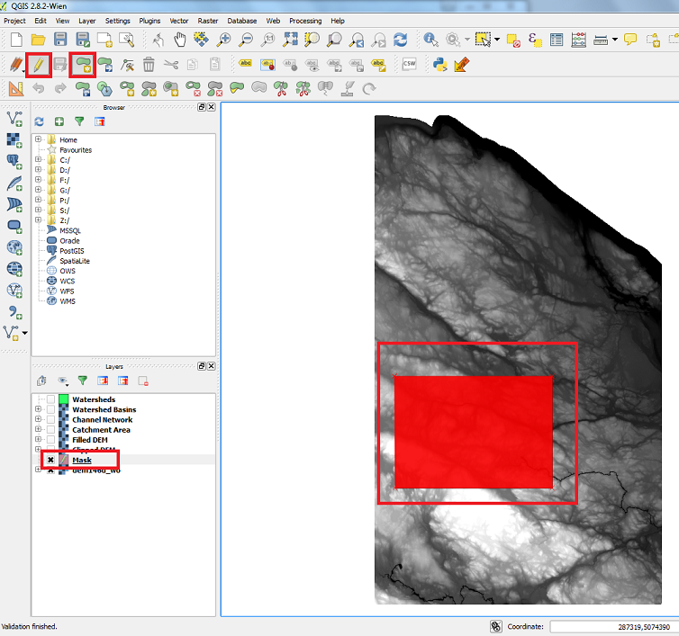
• With the Mask layer created, you will first want to single click on it in the QGIS table of contents on the left side of the screen.
• From there, either right click it or click the pencil near the top of the screen to Toggle Editing.
• After that, click on the button with a red box around it next to the pencil at the top to add a feature (draw a shape).
• Choose the area you want to clip the DEM down to and draw a box around it clicking at each corner and then right clicking to finish the box.
• Finish by Toggling Editing off by re-clicking the pencil at the top and saving your edits.

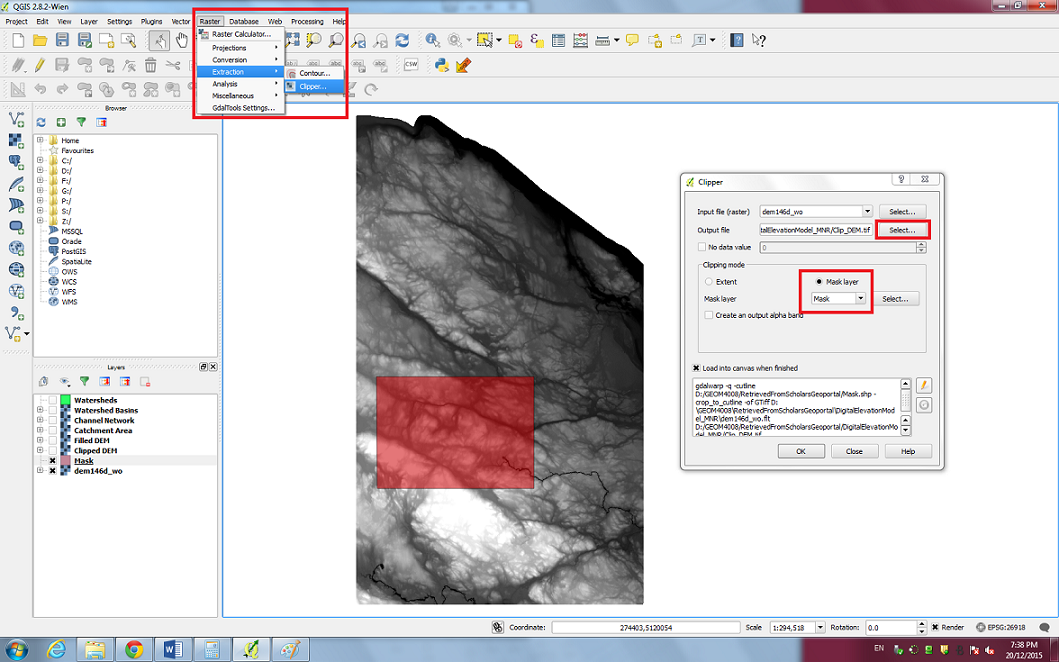
• With the Mask created and saved, go to Raster --> Extraction --> Clipper and in the algorithm box, change the same things I have changed in the figure below (highlighted with a red box).

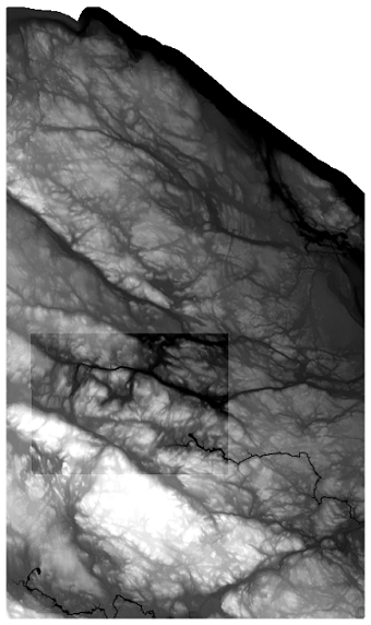
• The resulting clip can be seen on top of the larger DEM in the image found below.

Creating the Model

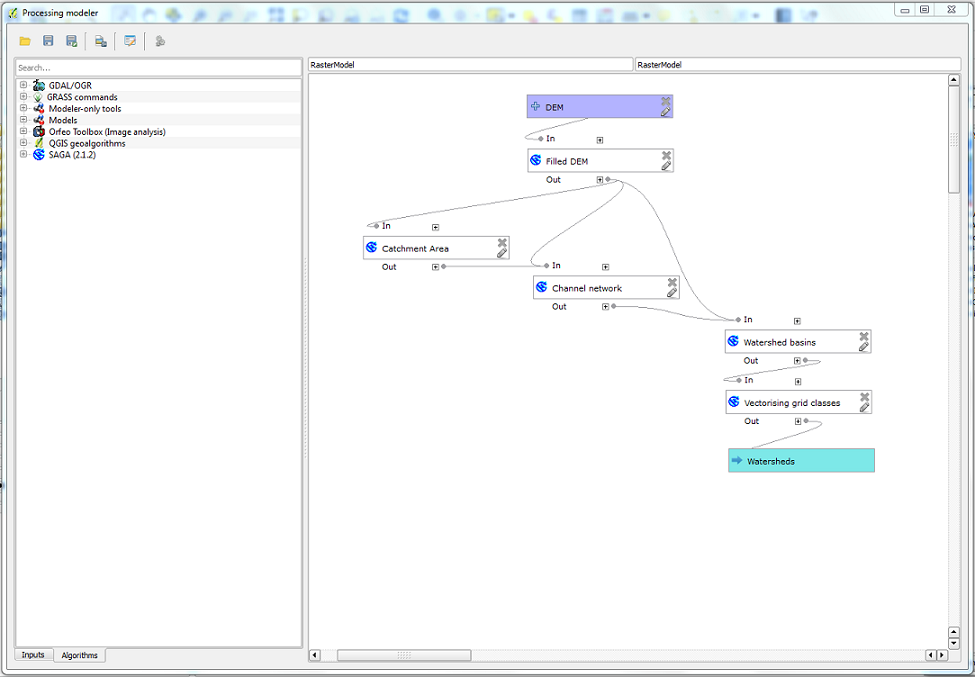
Below you will find the final appearance of the Raster Model since the steps for making one were covered in the vector tutorial above. With that being said, the input parameters for each of the algorithms used in this model can be found in the subsections below.

NOTE: When searching for algorithms, remember that all the algorithms chosen below come from SAGA.

Fill Sinks

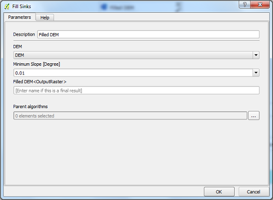
In order to create a "cleaner" DEM, the first algorithm used is the Fill Sinks which helps to removed the local depressions in the DEM.

• Using the Fill Sinks Saga algorithm, set the DEM input parameter as the clipped DEM.

Catchment Area

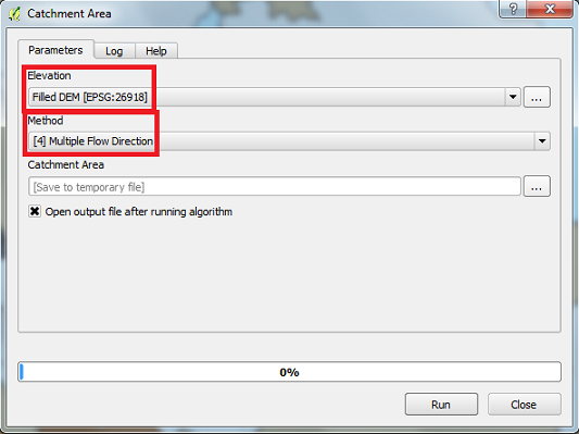
In order to create a Channel Network, we are required to first produce a Catchment Area raster.

• Using Saga's Catchment Area Algorithm, set the Filled DEM as the Elevation input and change the Method to Multiple Flow Direction.
• Play around with the Catchment Area methods as you please.

Channel Network

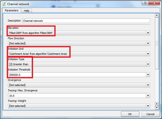
With the DEM filled and the Catchment Area made, we can now create a Channel Network.

• Following the input parameters found in the image below, make sure to use the Filled DEM and the Catchment Area as the Initiation Grid.
• The Initiation Type and Thresholds were chosen based on trial and error and decided based upon the fact that these options had a strong amount of channel delineation without too much detail.
• I advice doing some trial and error testing ahead of time (before working with a model) since for each DEM, these will differ.

Watershed Basins

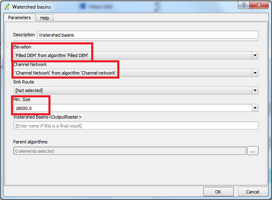
• Using the newly created Channel Network and the Filled DEM, we will now produce the Watershed Basins Raster.
• For this, trial and error was also used to determine a reasonable number of output watersheds. This varies highly from DEM to DEM, therefore do quite a few tests first.

Vectorising Grid Classes

With the watersheds delineated in raster format, this algorithm allows for the creation of the same watersheds in vector format.

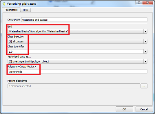
• Use the raster watershed basins as the grid
• Change the Class Selection to All Classes and set the Class Identifier to 1.0 (will not run if class identifier is 0)
• Keep the Vectorised class as One Single (Multi-)Polygon Object
• Since this is the last step of the model, set an output vector.

Output

• Before running the model, make sure everything is saved and double check the algorithm inputs.

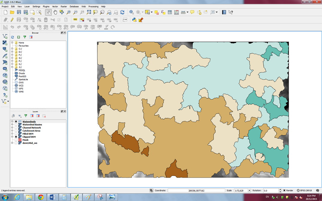
• The output watersheds using the steps above is shown below.

NOTE: Symbology is arbitrary and has no real significance.

Executing Models as Batch

• If you want to perform a model on various data sets at once (ex: wanting to create a watershed map for many DEM's), there is a way to run the models as a batch.
• To do this, first add your model through the processing toolbox (Processing Toolbox --> Models --> Tools --> Add Model From File) - a warning message might say that it cannot read the file but that is a lie.
• Navigate to the newly added model back through the Processing Toolbox and right click on it.
• From here you can run it, edit it or delete it, but you can also "Execute as Batch", allowing for multiple inputs and multiple outputs in one go.

Conclusion

After working with the QGIS Graphical Modeler, I can confidently say that it is very powerful and performs very well for all types of workflows. Although the models chosen above were arbitrarily chosen for demonstration and therefore have little real-world meaning, I hope that they help those reading create exactly what they were looking for. You stay classy San Diego.

Helpful Links & References

• QGIS Home Page: http://www.qgis.org/en/site/

• QGIS Graphical Modeler Documentation: http://docs.qgis.org/2.8/en/docs/user_manual/processing/modeler.html

• All Carleton Univeristy Tutorials: http://gracilis.carleton.ca/CUOSGwiki/index.php/Main_Page

• Scholars Geoportal: http://geo2.scholarsportal.info/