Coastal Flooding Assessment of Prince Edward Island using a 3D Model in QGIS

Introduction

preview of regional context

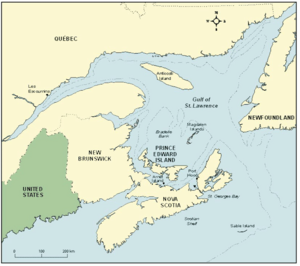
Over the past decades, global warming has become a prominent concern for environmentalists and lobbyists alike due to its impact on geological, atmospheric, and oceanic ecosystems. Human activities such as burning fossil fuels, clearcuttings, and overgrazing have been observed to influence the climate and increases Earth's surface temperature. This rise in ambient temperature increases the risks and probabilities of natural disaster occurrences on a global scale. This analysis focuses on assessing coastal flooding impacts surrounding the municipality of Charlottetown, Prince Edward Island (PEI). Prince Edward Island will be our designated area of interest (AoI) due to it's location within the Gulf of St. Lawrence and also resides beside the Northumberland Strait. As an island with a vast, low-lying coastline, PEI is highly vulnerable to the storm surges and sea-level rise that cause coastal flooding.

Coastal flooding is a sudden and abrupt flow of the coastal environment caused by a short-term increase in water level due to storm surge and extreme tides. It takes place when seawater flows over low-lying land that is normally dry and exists near the coast.

The objective of the tutorial is to illustrate the effectiveness of a 3D map for coastal flood risk assessment along with important information that can be extracted from it.

Software Requirements

In order to begin the tutorial, download the QGIS software package from the following link (https://www.qgis.org/en/site/ ). This tutorial was created using QGIS version 3.34.1 and updated to version 3.40.11 LTR. The latest version of QGIS is freely available for Windows, MacOS, Linux and Android.

Data

The raster data used for this analysis was obtained from High Resolution Digital Elevation Model (HRDEM) - CanElevation Series, produced by Natural Resources Canada for the city of Charlottetown. The dataset is hosted on the Open Data Canada website, with additional vector data retrieved from the Government of Prince Edward Island Open Data portal website.

Download instructions are provided in the section below.

Downloads

Charlottetown Digital Elevation Models Data

High Resolution Digital Elevation Model (HRDEM) - CanElevation Series

1. Click on the following link. This will take you to the directory where all of the DTM data is stored for the UTM 20 Zone. (Note: it may take some time to fully load the page)

2. Use the find function (Ctrl + F) to find each of the four images listed below which spans the area of interest.

dtm_1m_utm20_w_0_111

dtm_1m_utm20_w_0_112

dtm_1m_utm20_w_1_111

dtm_1m_utm20_w_1_112

3. Likewise, the following link will take you to the directory where all of the DSM data is stored for the UTM 20 Zone. (Note: it may also take some time to fully load the page)

4. Once again, use the find function to locate each of the four images listed below which spans the area of interest.

dsm_1m_utm20_w_0_111

dsm_1m_utm20_w_0_112

dsm_1m_utm20_w_1_111

dsm_1m_utm20_w_1_112

5. Create a new folder on your computer named "Raw Data", in the "Raw Data" folder create two sub-folders named "Vector Data" and "Raster Data" which will be used to store the vector and raster data respectively. You can also split the terrain and surface models into their own separate folder as well if you'd prefer.

Charlottetown Vector Data

1. Click on the following links and download the data as .shp files (a .zip file will be downloaded)

Roads: This is a line layer of the road network in Prince Edward Island.

Coastline Boundary: This is a polygon layer that spans the coastline surrounding Prince Edward Island.

Civic Communities: This is a polygon layer of communities in Prince Edward Island.

2. Extract the .zip files downloaded to the subfolder named "Vector Data".

3. As for the buildings data. It was obtained from here: (https://osmbuildings.org/data/) in the form of GeoJSON, due to the fact it can attribute a height measurement for each building which is important for 3D analysis.

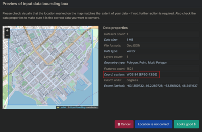
4. Convert the GeoJSON to shapefile using this website: (https://mygeodata.cloud/converter/geojson-to-shp). Ensure the coordinate system is the same as the image below (EPSG:4326), then click the "Convert" button and download the ESRI shapefile (.shp).

QGIS Methods and Instructions

Importing and Merging

Step 1.

• Open QGIS and create a new project.
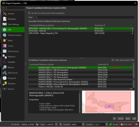
• Before any further geospatial analysis, the coordinate system of the project was set to NAD 1983 CSRS Prince Edward Island. Although the coordinate system of other layers should be different else they will not be displayed on the map.
• Locate the folder where the vector and raster data were saved by making use of the browser. Highlight all 4 raster data and add them to the project. Once this is done, add the required vector data such as buildings, road network, civic community zones and 2000 coastline boundary.
• When adding the the building and road network shapefile, a pop window might appear, select the first option and click Ok.
• If the steps above were followed correctly, the projected coordinate system of the project should be the same as the image below. This means the environment has been successfully set up for analysis. Raster and vector data used should have an Assigned Coordinate Reference System (CRS) of EPSG:4326 - WGS 84.

Rasters Prep

Step 2.

• Use the merge tool (Raster -> Miscellaneous -> Merge) to combine the dsm & dtm .tif files into two working raster images.
• In the merge tool window, select the four .tif files from either dsm or dtm groups through the Input Layers selection, directly under the Parameters tab.
• Under the Merged heading select the Save to File… option, give the output a name and save it in your working folder.
• Once the layers have been selected, click Run in order to merge the files.

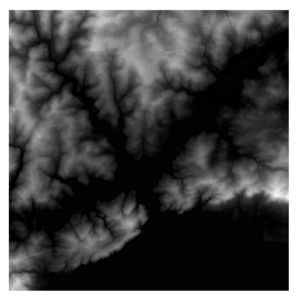
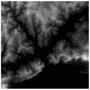
• The merged file should look similar to the final image below:

Select Feature

Step 3.

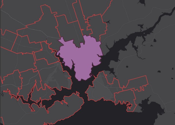
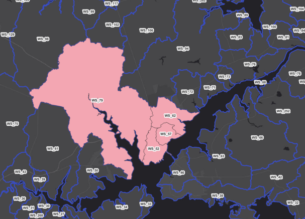
• The first operation to be done before clipping is extracting the city of Charlottetown from the Community Polygon layer and Charlottetown's shoreline from the Coastal Boundary layer using the watershed label id WS_79, WS_52, WS_57, and WS_62. This is done by making use of Select Features option in the toolbar.
• The selected features are exported by right-clicking on the layer then selecting Export -> Save selected features as. A window will pop up that request for a filename, in order to properly save the selected feature as a shapefile.
• Choose a name for the shapefile then select Ok.
• The result of the selection should reflect the image below.

Clipping

Step 4.

• The Community Polygon shapefile takes into account docks that are situated around the coast of Charlottetown. In order to get rid of this part of the shapefile, it has to be clipped using the Coastline Boundary shapefile.
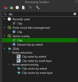
• There are different ways to access the Clip tool in QGIS. For this analysis it was done simply by making use of the search bar under the Processing Toolbox (Ctrl + Alt + T) which will be located at the right side of the work environment in QGIS.
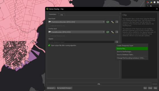
• Type Clip in the search bar and select the first option under Vector Overlay as shown in the image below, or find it under Vector -> Geoprocessing tools -> Clip.
• Once the tool is opened, set the Input layer to the municipality district shapefile that was extracted using the Select features in Step 4 and Overlay Layer set to the Coastline Boundary shapefile.
• Ensure to save the result of the clip by selecting Save to File then click Run.
• An error might be encountered after running the clip. To solve this issue, select Do not Filter (Better Performance) under the Advanced Options icon for both layers as shown in the image below, then click Run again.
• The road network is also clipped to cover only the city of Charlottetown. Set the parameter of the Clip tool as follows; Input layer as Road Network shapefile and Overlay layer as the output shapefile of the clip executed earlier, then click Run.

Creating AOI

Step 5.

• Create a polygon that can be used to clip the raster layer and also further concentrate the study area to the coast of Charlottetown.
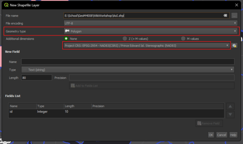
• Using the toolbar, select Layers -> Create Layer -> New Shapefile Layer.
• A window will pop up, which requires a filename for the new file, AOI (Area of Interest) would suffice for the purpose of this tutorial.
• Select Polygon as the Geometry Type and ensure the co-ordinate system is NAD 1983 CSRS Prince Edward Island (EPSG: 2954) then Click Ok. A new layer named AOI will appear in the Layers section at the bottom left of the work environment.
• Right click on the AOI layer and once this is selected, navigate to the top panel and select the Toggle Editing icon , then find the Add Polygon Feature button off to the right.
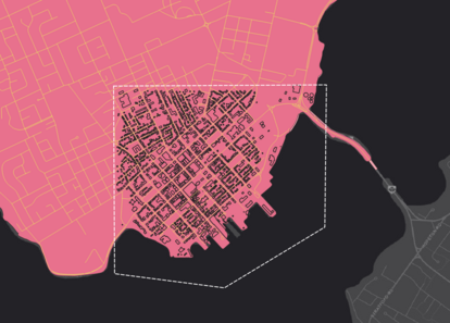
• Draw a border that roughly spans infrastructure (buildings and road network) close to the coast of Charlottetown when complete, right click on the outline and a new window will pop up that request for ID, type 1 then click Ok.
• If all steps are followed properly, the result should be similar to the image on the right. Do not forget to click Save layer edits and un-toggle the editing.

Final Clipping

Step 6.

• A second round of clipping is done on the road network and buildings shapefile, since the analysis is not based on the overall area of Charlottetown. We will make use of similar steps in Step 4, the only difference is the Input layer and Overlay layer selection.
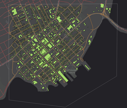
• For the road network, set the Input layer to the Buildings shapefile and Overlay layer to the AOI shapefile created in Step 5, select Save to File and give the shapefile a name then click Run.
• For the buildings, set the Input layer to the Clipped Road Network from Step 4 and and Overlay layer to the same AOI shapefile, select Save to file and give the output shapefile a name then click Run.
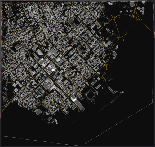
• The final output should look like the image shown below.

Step 7.

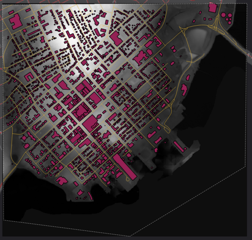
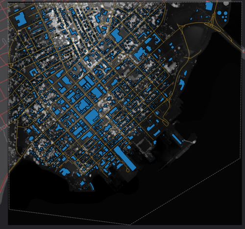
• The merged rasters created in Step 2 will be clipped using the AOI shapefile. This will be executed with the help of Clip by Mask Layer tool.
• In the search toolbar of the Processing Toolbox, type Clip and select the Clip by Mask Layer under Raster Extraction, or alternatively Raster -> Extraction -> Clip Raster by Mask Layer.
• Once the tool is opened, set the Input Layer to the merged rasters and Mask Layer to the AOI shapefile, finally select Save to file and give the output rasters a name then click Run.
• The final output should look similar to the Terrain model on the left and the Surface model on the right shown below.

Raster Calculator

Step 8.

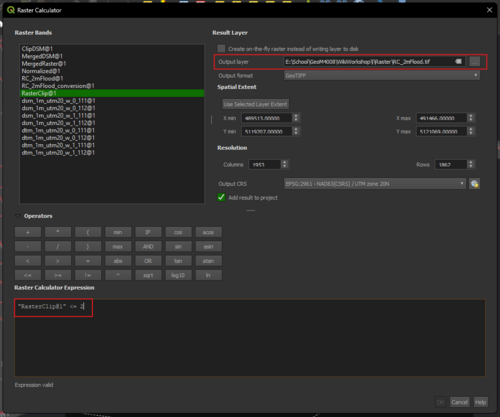
• Raster calculator is commonly used to extract all elevation pixels below or above a certain threshold. For the purpose of this tutorial, the threshold for the flood level simulated will be 2m.
• Using the toolbar, select Raster -> Raster Calculator.
• Select the merged dtm raster that was clipped in Step 7.
• Input the expression of your clipped merged dtm in the Raster Calculation Box with a value smaller than or equal to 2 (<= 2), create a name for the output file and ensure it is in .tif format.
• Click Ok and run the expression.
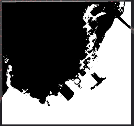
• The raster image below meets the threshold that was set using the raster calculator.

Step 9. When inspecting the attribute table from the OSM Buildings dataset we collected earlier, we can identify that the height column is very depopulated, with only a select few buildings having accurate height measurements. To fix this issue, we are going to use manipulate the surface model to attain an estimated building height by creating a normalized surface model.

• By this point you should've performed the same steps to the dsm as you did in the previous steps with the dtm so we'd result with both dtm & dsm merged into their respected models and clipped to the municipality of Charlottetown.
• To create the Normalized dsm, use the raster calculator tool (Raster -> Raster Calculator) and subtract the DTM from the DSM, similar to step 8 above, and should provide you with a raster similar to the one below.

Changing NoData Value

Step 10.

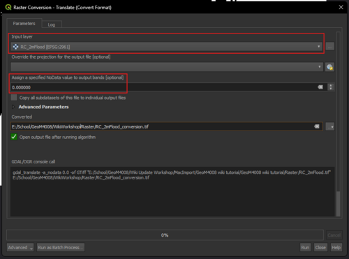
• Changing NoData values allows you to set a specific value in the raster dataset to be transparent. This is useful for visualization purposes, as it makes it easier to distinguish between valid data and exclude certain areas from analysis.
• Using the toolbar, select Raster -> Conversion -> Translate.
• Set the parameters as follows: Input Layer should be set to the raster obtained from Step 8, NoData Value should be set to 0.
• Finally select Save to file and give the output raster a name then click Run.

Polygonize

Step 11.

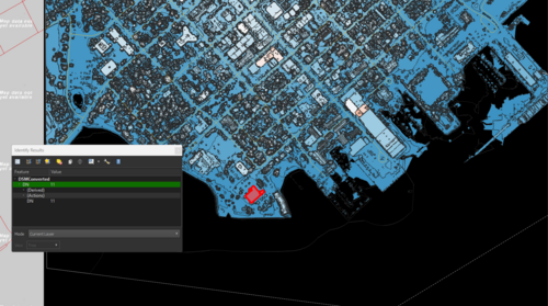
• With the Normalized surface model, we can polygonize the resulting raster (Raster -> Conversions -> Polygonize (Raster to Vector)) to identify the height values of every pixel within our AoI with the Identify Features tool . By inspecting one of the surrounding buildings along the coast, we can now get an estimate to the heights of each & every building in our AoI as shown in the right side panel. in this case, the highlighted building should have an estimated height of 11 meters as shown below.

• These height values can be further isolated and averaged per building with the help of our collected OSM building shapefile by using the Zonal Statistics processing tool within the processing toolbox. Using the clipped building shapefile as the Input Layer, the Normalized dsm as the Raster Layer, changing the Statistics to Calculate parameters to only capture the mean of the polygons, and saving the output.
• The shapefile created by the zonal stats tool will now include the average height measurements in a new column within the attribute table and we can continue with the next steps.

Symbology

Step 12.

• An important aspect of the 3D analysis are the buildings. For this reason, the symbology should be configured properly to have a good representation of height difference across the buildings in the area of interest.
• Right click on the Buildings shapefile, select Properties then click Symbology on the window that pops up.
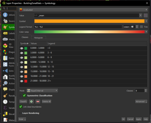
• Change the type of the symbology to Graduated and the Value parameter to the _mean attribute of the buildings.
• Edit the values represented by the symbology to be similar to the second image below, then click Apply to save the changes.
• Click Ok to close the window.
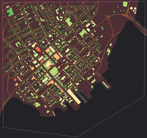
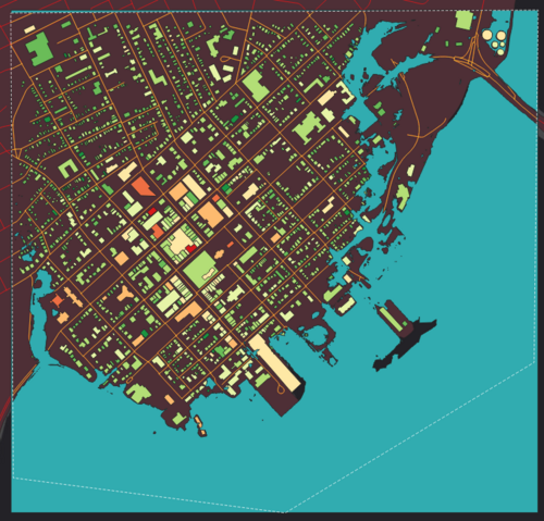
• After the changes are made, the buildings should be grouped with the colors selected based on their height (m). Refer to the map below for an example.

Qgis2threeJS

Step 13.

• Finally, here is the fun part of the analysis.
• Using the menu toolbar, select Plugins -> Manage and Install Plugins. A new window will pop up.
• Click the All section and type: Qgis2threeJS then select Install plugin.
• Note: The Install plugin option is replaced with Reinstall plugin if its was previously installed.
• If the plugin was successfully installed, it should appear in the vector toolbar with this icon:

• Click the icon and a new window should pop up.
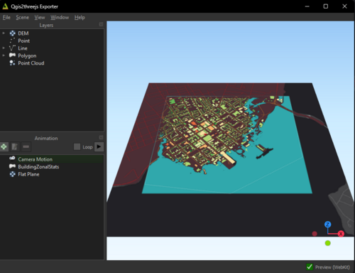
• In the Layers section of the tool, check the Flat plane within the DEM dropdown and the Buildings shapefile obtained from the zonal statistic section, it should automatically import the 2D map and shapefile into the 3D work environment. Both layers should be available in the Animation section as shown in the image below:

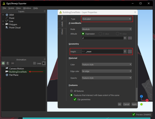
• Right click on the Buildings shapefile and select Properties.
• Once the window pops up, set the Type to Extruded and Height to the height attribute of the Buildings shapefile, then click Apply followed by Ok to close the window. Illustrated in the image below:

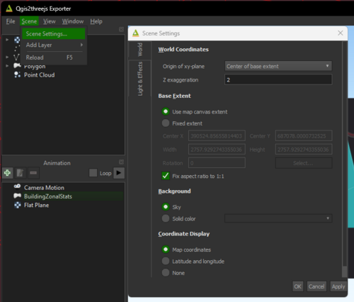
• Optionally, you can increase the extent of extrusion for the buildings by selecting Scene -> Scene Settings. Increase the Z exaggeration to 2.0, then click Apply followed by Ok to close the window :

• To finalize the 3D map, a legend and north arrow needs to be added.
• In order to add a north arrow, select View -> Widgets -> North Arrow in the toolbar. Make sure Enable North Arrow is checked, then click Apply followed by Ok to close the window:
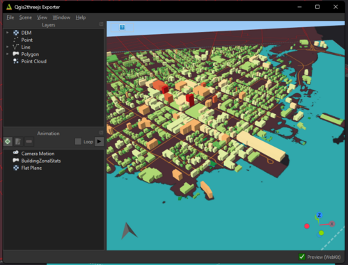
• Create a legend for the 2D map. Go back to the 3D environment, click View-> Widgets->Header/Footer labels. A window should pop up that gives the option to create a header or footer. In the header section, type: <img src="qgis_legend.png" alt="Legend">. Lastly, click Apply followed by Ok to close the window. If done correctly, a box with a question mark should appear at the top left of the screen as shown in the image on the right:
• The [?] box searches for an image of the legend within the destination folder chosen above. If the legend doesn't auto-populate when exporting to the web (File -> Export to Web), a quick fix is to export a image of the legend through printing a layout as a .png, naming it "qgis_legend", and placing the image inside the files' saved location above.

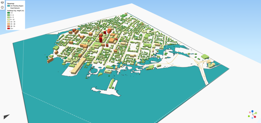
• Final product:

• The tutorial ends here

Conclusion

To sum it all up, based on the map above it can be concluded that buildings that are colored in green are at high risk and susceptible to flooding, especially those situated near the coast. Buildings that are colored in the yellow spectrum are medium risk depending on their proximity to the coast. Lastly, buildings that are colored in red are low risk due to them having the highest elevation. There are outliers, as some of buildings may not have a uniform ceiling height, like an antenna or tower protruding above the rest of the building, which can lead to skewing the average height of the building. The tall buildings in our AoI could serve as an evacuation muster point, in the case of severe flooding. This is one of the benefits of making use of a 3D map, especially from the perspective of a city planner.

References

“Step-By-Step: Use of Digital Elevation Data for Storm Surge Coastal Flood Modelling | UN-SPIDER Knowledge Portal.” Www.un-Spider.org, www.un-spider.org/advisory-support/recommended-practices/dem-storm-surge-coastal-monitoring-airbus/step-by-step.

“Management of Coastal Flooding.” Www.coastalhazardwheel.org, www.coastalhazardwheel.org/coastal-flooding/.