Comparative Analysis of Cost Path Analysis In Grass GIS and ArcMap

Introduction

About The Tutorial

Cost Path analysis allows us to consider a variety of cost factors that may be present in traversing a landscape. These factors may represent a variety of situations from financial cost to risk to associated difficulty in traversing terrain, slope or landscapes.

ESRI presents a solution to determining optimal cost path across a cost surface in its proprietary software ArcMap, however such a solution can also be achieved using Free and Open Source Software for Geospatial (FOSS4G) tools. In particular the FOSS4G suite GRASS GIS will be used to replicate the results of the same procedure in ArcMap. Both processes will be worked through and compared in the tutorial that follows.

Little Red

In the spirit of the European fairytale Little Red Riding Hood the goal of this lab will be to find the optimal path to Gramma's House. The cost factors used in determining optimal path will be slope, and land cover type as Little Red will also be trying to avoid the wolf. Based on this story framework cost will be assigned based on slope steepness and landcover type, which will permit the determination of Little Red's path if she only seeks to avoid slope or multi-factored cost models if she also seeks to avoid the wolf as well. This lab concept is used with permission of its creator Dan Patterson.

ArcMap

About ArcMap

ArcMap is the proprietary GIS Software of the company ESRI and is a popular commercial solution used by companies to perform spatial operations.

Setup and Data

Open ArcMap and create a new map layout, making sure to set the workspace to known folders.

The following data files used are:

• 1. littlered.shp - The start location of little red.
• 2. gramma.shp - End location Gramma's cottage.
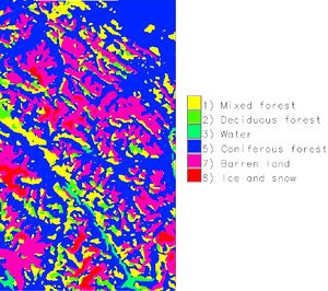
• 3. landcover.shp - The land cover types present which are used to determine likelihood of encountering the wolf.
• 4. elevation.shp - Elevation points for the area.
• 5. AOI.shp - Area of interest polygon that defines study area.

Add all of the above layers to the data frame.

Interpolation

In order to obtain the slope factor we first need to create a Digital Elevation Model (DEM) from our elevation points.

The DEM will be interpolated using the Inverse Distance Weighting (IDW)method and will be created with 500 m resolution. This is obtained with ArcMap's IDW tool.

ArcToolBox/SpatialAnaylstTools/interpolation/IDW

The Z field is contained in the attribute elevation, the output cell size will be 500 m and variable search radius of 12 points (default value).

Figure :Screenshot of IDW Tool

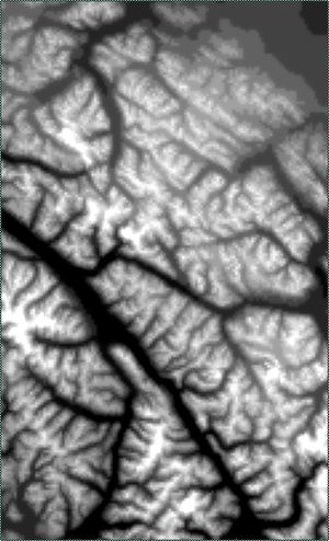
Figure : Digital Elevation model of AOI from IDW Interpolation

Determining Slope

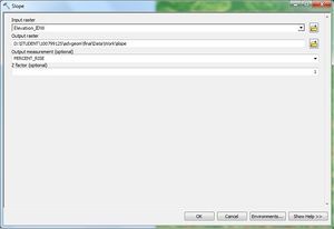
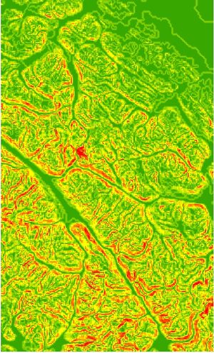
A Slope raster is created using the Slope tool of ArcToolbox, this will use the previously created DEM and give slope in percent rise with a z factor of 1. The result raster shows slope in percent from green to red where red is the maximum slope.

ArcToolBox/SpatialAnaylstTools/Surface/Slope

Figure : Slope Tool

Figure : Percent Slope of AOI

Polygon to Raster

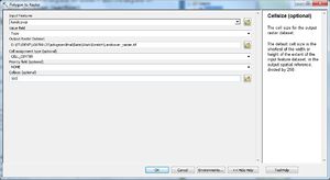
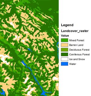
The land cover polygon must be converted to raster in order for it to be used for cost anaysis. The type conversion is done using the Polygon to Raster tool in ArcToolbox where the raster value assigned will be based on the "type" field such that polygon value that overlaps the middle of each 500 m cell defines the land cover assigned.

ArcToolBox/ConversionTools/ToRaster/PolygontoRaster

Figure : Polygon To Raster Tool

Figure : Raster of Landcover

Cost Reclassification

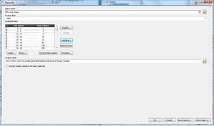
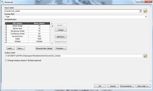
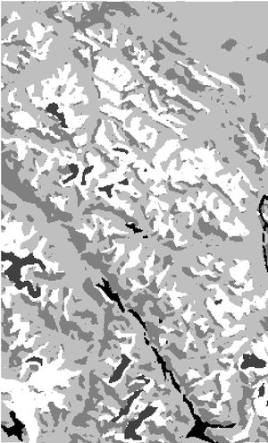
Both the Slope Raster and Land cover raster must be reclassified with cost values based on the percent slope and land cover types respectively. As per the originally specified difficulty and likelihood of wolf factor outlined in the introduction above each raster is re-classed with the Reclassify tool. The reclassification will be based on the value and Type fields for slope and land cover respectively. Cost is shown in the results over white to black where black is the maximum cost.

ArcToolBox/SpatialAnaylstTools/Reclass/Reclassify

Figure : Reclassify Tool with: Slope parameters, Land cover parameters

Figure : Raster of slope cost, Raster of land cover cost

Cost Distance and Back link

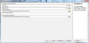
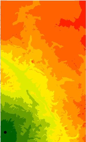
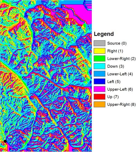
The Cost Distance raster tracks the cumulative cost of traveling from each cell to the source (destination). For this example the destination/source will be Gramma's cottage as denoted by a black point on each map below. We have the option of setting an output location for the back link raster or this can also be created independently using the back link tool as it will be required to calculate optimal cost path.

The cost distance raster shows cumulative cost from a given cell to the source by the cheapest path as determined by the input cost grid. The back link raster gives the direction of movement from each cell toward the source on the least cost path as determined by the cost grid.

ArcToolBox/SpatialAnaylstTools/Distance/CostDistance

Figure : Cost Distance Tool

Figure : Cost Distance and Backlink Raster of Slope Cost

Cost Path

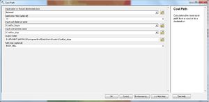
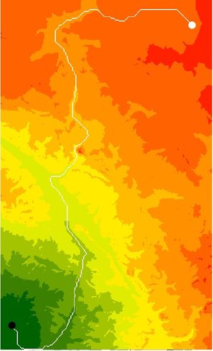
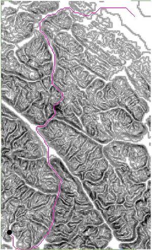
The cost path analysis finds the least cost path between the destination(Little Red) and the source (Gramma's Cottage) based on the cost distance and back link rasters. The following cost path is based on the slope only example that has been demonstrated thus far. The cost path tool generates only the polyline path, this polyline has been laid over each of the slope cost distance and slope cost for comparison.

Figure : Cost Distance Tool

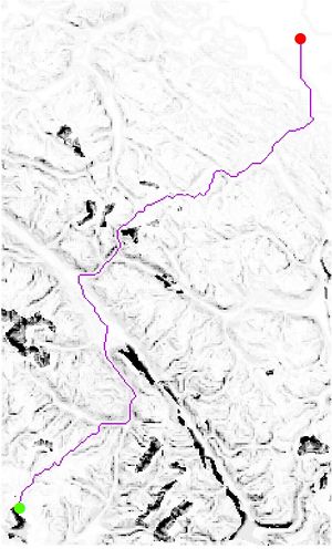
Figure : Cost path for Slope Factor overlaid on slope cost distance, the slope cost grid.

Multi-Factor Cost Models

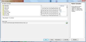
Cost can be calculated using combination models of more then one cost factor. Two ways this can be done is with additive or multiplicative model where two cost rasters are combined. This can be performed in ArcMap using the raster calculator on each of the determined cost rasters as follows:

• 1. Additive Model= slope_cost + landcover_cost
• 2. Multiplicative Model= slope_cost * landcover_cost

ArcToolBox/SpatialAnaylstTools/MapAlgebra/RasterCalculator

Figure : Raster calculator to construct multiplicative, additive model.

Using these new cost rasters the cost distance, back link and finally cost paths can be determined. The resulting optimal cost paths have been included below overlaid on their determinate cost grids.

Figure : Raster optimal cost path overlaid on cost distance raster for multiplicative and additive cost model respectively.

GRASS GIS

About GRASS

The Geographic Resources Analysis Support System (GRASS) is a Free and Open Source Software for Geospatial operations (FOSS4G) software suite. GRASS is free open source used in a variety of GeoSpatial operations and has been supported and developed with its community to perform a growing list of geospatial tasks.

Intro to GRASS GIS

GRASS GIS is advantageous in its command line operation as complex operations can be constructed and completed by a single line of instruction with appropriate flags and parameters given. These commands can be built using the GRASS Guided User Interface (GUI) via menu based navigation and selection. The appropriate command structure will be provided with some basic GUI guidance.

Setup and Data

Open ArcMap and create a new map layout, making sure to set the workspace to known folders.

The following data files used are:

• 1. littlered.shp - The start location of little red.
• 2. gramma.shp - End location Gramma's cottage.
• 3. landcover.shp - The land cover types present.
• 4. elevation.shp - Elevation points for the area.
• 5. AOI.shp - Area of interest polygon that defines study area.

Arc to GRASS

As the original data used is presented in ESRI's shapefiles (.shp)or once developed further Arc/Info Binary Grids these files will have to be either converted or opened in a particular manner to be used in GRASS. The methods by which ESRI's files can be accessed with GRASS are summarized below. ESRI's file formats are GDAL (Geospatial Data Abstraction Library) compliant and therefore can be abstracted and transferred between GIS Suites. By extension non raster vector features are supported by the OGR simple features library.

Shapefiles

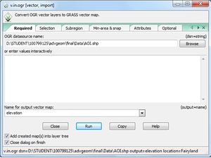
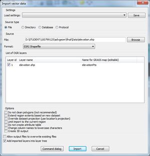
v.in.ogr converts OGR compatible vectors to GRASS Vectors. Shapefiles may be directly referenced by path under the dsn parameter, and if the name for a new location is specified (under the optional tab) a new location is created based on the imported extent.

This can be done using the command:

v.in.ogr dsn=D:\STUDENT\100799125\advgeom\final\Data\AOI.shp output=AOI location=FairyLand

For straight vector import without creating a new location this would become:

v.in.ogr dsn=D:\STUDENT\100799125\advgeom\final\Data\Elevation.shp output=elevation

This can be repeated for each required vector shapefile by selecting the appropriate file paths and output names.

Figure : Import of vector shapefile to define location, import of vector shapefile

Raster Grid

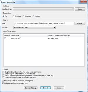
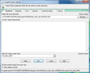
r.in.gdal converts an ESRI Arc ascii raster GRID file into a GRASS compatible binary raster layer. ESRI's Grid files are GDAL compliant and as such can be easily imported into GRASS using the following command structure, where input and output file names are specified. Within the folder of an ESRI raster the w001001.adf file is that which contains the full raster and should be selected for import.

r.in.gdal input=D:\STUDENT\100799125\advgeom\final\arc_elev_idw\w001001.adf output=Arc_Elev_IDW

Figure : Import of Arc raster

Interpolation

In order to obtain the slope factor we first need to create a Digital Elevation Model (DEM) from our elevation points.

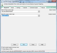
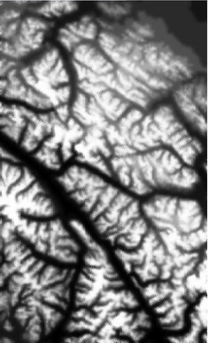
In GRASS IDW Interpolation from elevation points is performed using the module v.surf.idw. For this and any raster operations that follow it is important to make sure we set our region cell size to 500 using: g.region res=500'.'

The DEM will be interpolated using the Inverse Distance Weighting (IDW)method and will be created with 500 m resolution. The interpolation values are contained in the table column ELEVATION, the output cell size will be that of the region and the number of interpolation points and power will be 12 and 2 respectively just as in ArcMap (default value).

In order to produce this DEM using IDW the following command is used:

v.surf.idw input=elevation@PERMANENT output=elevation_IDW column=ELEVATION

Figure :Screenshot of IDW Module

Figure : Digital Elevation model of AOI from IDW Interpolation

Determining Slope

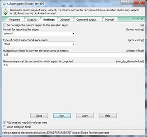
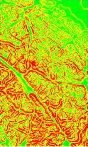
A Slope raster is created using r.slope.aspect which is a terrain analysis tool. This will use the previously created DEM and give slope in percent, with a multiplicative factor of 1. The result raster shows slope in percent from green to red where red is the maximum slope.

Slope in percent is calculated with r.slope.aspect using the following command:

r.slope.aspect elevation=elevation_IDW@PERMANENT slope=Slope format=percent

Figure : Slope Module

Figure : Percent Slope over AOI

Polygon to Raster

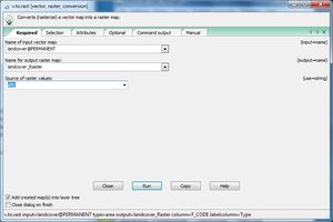
The land cover polygon must be converted to raster in order for it to be used for cost anaysis. The type conversion is done using the v.to.rast module in vector/map_type_conversions. The raster value assigned will be based on the numeric "F_CODE" field such that polygon value that overlaps the middle of each 500 m cell defines the land cover assigned. This conversion is performed using the following command:

v.to.rast input=landcover@PERMANENT type=area output=landcover_raster column=F_CODE labelcolumn=Type

Figure : Polygon To Raster Tool

Figure : Raster of Landcover

Cost Reclassification

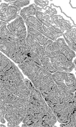
Both the Slope Raster and Land cover raster must be reclassified with cost values based on the percent slope and land cover types respectively. As per the originally specified slope difficulty and likelihood of wolf factor outlined in the introduction each raster is re-classed with the Reclassify tool. The reclassification will be based on the value and Type fields for slope and land cover respectively. Cost is shown in the results over white to black where black is the maximum cost.

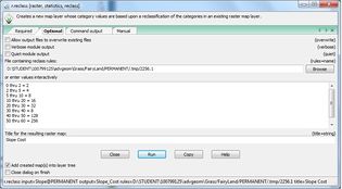
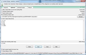
In GRASS this is done with r.reclass under raster/change categories and labels/reclassify. This is performed using the following sample command.

r.reclass input=Slope@PERMANENT output=Slope_Cost rules=Temporary/File/Path title=Slope Cost

The following are the reclass rules used to impose cost on categories.

Reclass Rules Slope

0 thru 2 = 2

2 thru 5 = 4

5 thru 10 = 8

10 thru 20 = 16

20 thru 30 = 32

30 thru 40 = 8

40 thru 50 = 128

50 thru 60 = 256

60 thru 100 = 512

Reclass Rules Land cover

1 2 = 75

5 = 50

7 = 10

8 = 500

3 = 1000

Figure : Reclassify Tool with: Slope parameters, Land cover parameters

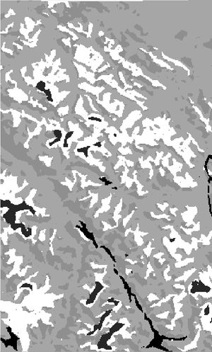
Figure : Raster of slope cost, Raster of land cover cost

Cost Distance

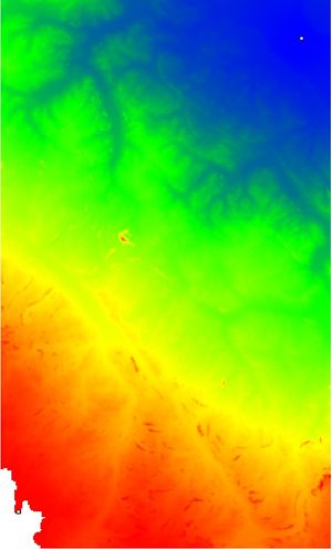
The Cost Distance raster tracks the cumulative cost of traveling from the start point to the stop point. For this example the stop point will be Gramma's cottage as denoted by a black point on each map below. The cost distance raster shows cumulative cost from the start point to the end point.

There are two obvious modules within Grass that could conceivably produce cost distance and direction rasters, those being r.walk and r.cost respectively. The r.walk module is constrained by its requirement of always considering elevation in its cost assessment, while this can be supplemented with an additional cost grid it is still a requirement. Another issue this presents is in that it restricts how multiple cost factors are combined as will be performed later in the tutorial. With that being noted this tutorial will use r.cost and its uni-grid cost dependence.

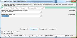
The r.cost module is found under the terrain analysis section of the raster menu. The r.cost module uses a cost grid to determine the cost of pathing from the provided start point (little red) to the provided stop point (Gramma's Cottage) which can be provided as raster or vector data. The R cost module is executed by the following command:

r.cost. input=Slope_Cost@PERMANENT output=slope_costDist start_points=littlered@PERMANENT stop_points=gramma@PERMANENT

Figure : R.Cost Tool with parameter

Figure : Cost Distance Raster

Cost Path

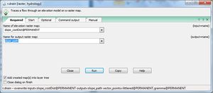
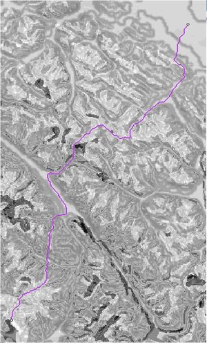
The r.drain module finds the least cost path between the start point (Little Red) and the end point(Gramma's Cottage) based on the calculated cost distance raster. The following cost path is based on the reclassified slope cost only example that has been demonstrated thus far. This module is performed with the following command where the Cost path grid from the previous step as well as the start and end points are given as input:

r.drain input=slope_costDist@PERMANENT output=slope_path vector_points=littlered@PERMANENT,gramma@PERMANENT

Figure : Cost Distance Tool

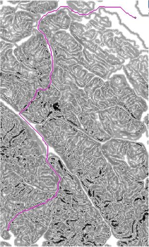
This produces a binary raster grid on cells on the optimal path and those which are not, for comparison with ArcMap results this can be converted to vector using the r.to.vect module with the correct input file and otherwise default variables. The resultant vector has been overlaid on the calculated slope cost grid.

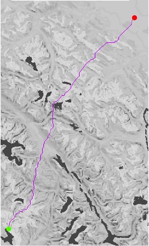
Figure : Cost path for Slope overlaid on slope cost grid.

Multi-Factor Cost Models

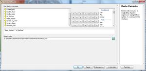
Cost can be calculated using combination models of more then one cost factor. Two ways this can be done is with additive or multiplicative model where two cost rasters are combined. This can be performed in GRASS using the raster map calculator on each of the determined cost rasters as follows:

• 1. Additive Model= slope_cost + landcover_cost
• 2. Multiplicative Model= slope_cost * landcover_cost

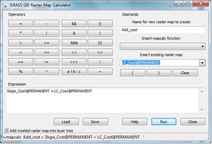
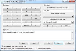
These calculations can be performed with the following commands:

• 1. r.mapcalc Add_cost = Slope_Cost@PERMANENT+LC_Cost@PERMANENT
• 1. r.mapcalc Add_cost = Slope_Cost@PERMANENT*LC_Cost@PERMANENT

Figure : Raster calculator to construct additive, multiplicative model.

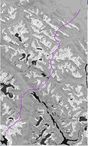
Using these new cost rasters, the cost distance and cost paths can be determined and converted to vectors. The resulting optimal cost paths have been included below overlaid on their determinate cost grids.

Figure : Raster optimal cost path overlaid on cost distance raster for multiplicative and additive cost model respectively.

Results

In order to compare results several steps can be taken. One such consideration which requires preparation is calculating the length of each determined path.

ArcMap

Using the conversion tools on the resulting cost path grid will allow us to convert them from raster to vector so we can take additional measurements. This is done with conversion tools/from raster/raster to polyline. Provided the input and output is given all the default variables will be sufficient for this conversion.

Once this is completed a new field must be created within the polyline's attribute table. This is done by clicking the dropdown arrow in the attribute table and selecting add field. This field should be of type double with precision 8 and scale 2 which defines the number of significant digits before and after the decimal place respectively.

By right clicking this new field we can calculate geometry on this field we can calculate the length in km.

GRASS

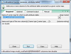
As our procedure in establishing the cost paths have already led us to convert to a vector it will now be necessary to add a new field to each of our lines and calculate the length. In order to add a field to a vector we will use the v.db.addcol module which allows us to add a column to a named vector with a given name and type as follows:

v.db.addcol map=muli_costPathV@PERMANENT columns=len double

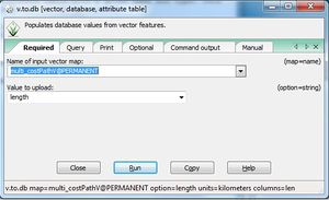
This should insert the desired column in our data table, once we have confirmed it is there we can use the new column to calculate the vector length using the v.to.db command, which is called with the option set to length, the units km with the map and column to use specified.

v.to.db map=multi_costPathV@PERMANENT option=length units=kilometers columns=len

Figure : Modules used for the creation and calculation of attributes.

Checking for equality

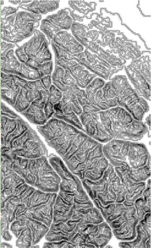
If we wish to compare the equality of any of the comparable grids we have devised in both ArcMap and Grass we can load the ArcMap Grid into GRASS using the r.in.gdal procedure discussed. In order to perform a cell by cell comparison we use the raster map calculator to directly check equality. An example of this would be the command as follows which will produce colored cells where the grids are equal and white cells where they diverge.

r.mapcalc Slope_CostTest=Slope_Cost@PERMANENT==Arc_Slope_Cost@PERMANENT

Slope only model

Figure : Optimal Cost path for slope factor as determined by ArcMap, GRASS GIS

Additive model

Figure : Optimal Cost path for additive model as determined by ArcMap, GRASS GIS

Multiplicative model

Figure : Optimal Cost path for multiplicative model as determined by ArcMap, GRASS GIS