Creating Interferogram for Mapping Earthquake Deformation by using Sentinel-1 Data in SNAP

Introduction

Radar is a form of active remote sensing in which the system produces its own electromagnetic signal, beams it at the target object, and measures the reflected energy. Spatial resolution of radar systems is dependent on the size of the antenna (aperture) used to generate the signal. Synthetic-aperture radar (SAR) refers to synthetically increasing the size of the aperture by combining a sequence of acquisitions. There are two values of importance for SAR imagery. The first is amplitude, which is a measure of the strength of the reflected signal and is related to how much energy was absorbed or reflected. The second is phase, which is related to the distance between the antenna and the object. Interferometric SAR (InSAR) refers to the method of combining SAR images of the same region taken at slightly different angles with the goal of extracting terrain information by determining the phase difference between the two images. The resulting data can be used to interferograms which have a wide variety of applications including monitoring natural hazards like earthquakes.

The European Space Agency (ESA) launched Sentinel-1, a two-satellite constellation, as part of the Copernicus Programme. Sentinel-1 operates in the C-band (~5-6cm) of the electromagnetic spectrum. This band can penetrate clouds allowing data to be collected in all weather conditions. Additionally, since SAR imaging does not rely on sunlight, data can be collected day and night, allowing for continuous collection.

This tutorial uses the opensource image processing software SNAP to create an interferogram. The interferogram is used to visually represent terrain deformation due an earthquake. Two examples of recent earthquake events have been provided.

Note: the data files used in this tutorial are quite large so it is suggested that this step be completed ahead of time as it may take a few hours to complete the downloads.

Background Information

The 7.8 magnitude 2016 Kaikoura earthquake in the South Island of New Zealand occurred two minutes after midnight on 14 November 2016 NZDT (11:02 on 13 November UTC). Ruptures occurred on multiple faults leading some experts to describe it as "most complex earthquake ever studied".

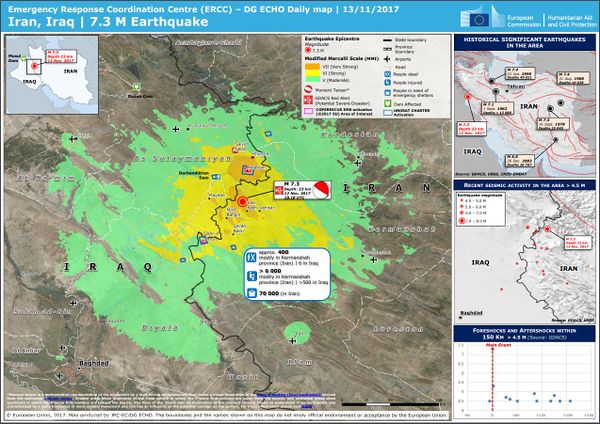
On 12 November 2017 at 18:18 UTC (21:48 Iran Standard Time, 21:18 Arabia Standard Time), an earthquake with a magnitude of 7.3 occurred on the Iran–Iraq border, with the Iraqi Kurdish city of Halabja, and the Kurdish dominated places of Ezgeleh, Salas-e Babajani County, Kermanshah Province in Iran, closest to the epicentre.

Interferometry refers to the technique of combining electromagnetic signals for the purpose of studying their interference patterns. In this case, the the phase signals of the SAR images taken before and after the earthquake events are combined. These interference patterns are converted into what is called an interferogram. After the signals related to the topography of the region are removed, the deformation due to the earthquake can be clearly observed.

Sentinel-1 Data and Software

The following data files will be used to create the interferograms in the tutorial. You will need to first register for a free EarthData account.

**Table 1: Data Acquisition**
Data	Data Time	Data Download Link
Before 2016 Kaikoura earthquake	2016 Nov. 03	download link Full name: S1A_IW_SLC__1SSV_20161103T072220_20161103T072250_013774_0161F9_2F68.
After 2016 Kaikoura earthquake	2016 Nov. 15	download link Full name: S1A_IW_SLC__1SDV_20161115T072214_20161115T072244_013949_016775_84CF.
Before 2017 Iran–Iraq earthquake	2017 Nov. 11	download link Full name: S1A_IW_SLC__1SDV_20171111T150004_20171111T150032_019219_0208AF_EE89.
After 2017 Iran–Iraq earthquake	2017 Nov. 17	download link Full name: S1B_IW_SLC__1SDV_20171117T145926_20171117T145953_008323_00EBAB_AFB8.

System Requirements	SNAP Download
Windows or Mac OS X Requires at least 16 GB memory RAM A Solid State Drive, as opposed to Hard Disk Drive, will speed up processing Close other applications Do not use the computer while a product is being processed Remove the previous product once a new product has been generated.	Sentinel-1 Toolbox - The current version is 7.0.0 (22.07.2019 13:30 UTC). Download Link (Version depends on your working environment!)

Data Processing

Step 1: Start software and open data

After you have successfully installed SNAP and downloaded the Sentinel-1 files above, open SNAP and load the images into the program by completing the following steps:
- Load data by navigating to File | Open Product | “yourzipfile.zip” and opening the .zip files that were just downloaded.
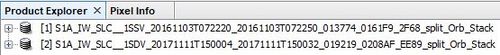
- click Open to add the data in SNAP. You can view your data in Product Explorer window where each available band in the dataset is listed.

Each band name is broken down as follows: Datatype_subswath_polarization

Where the data type refers to the real (i), imaginary (q), or complex (Intensity) data. The IW2 subswath and VV polarization bands will be used to create the interferograms.

Steps2: Split data

The Split tool is used to select the bursts required for the analysis. Bursts correspond to a region of the image, the required bursts for this analysis are provided below. The tool also isolates the desired subswath and polarization band combinations.

For data of 2016 Kaikoura earthquake
- we use IW2, VV and burst from 6 to 9 for S1A_IW_SLC__1SSV_20161103T072220_20161103T072250_013774_0161F9_2F68.
- then use IW2, VV and burst from 7 to 10 for S1A_IW_SLC__1SDV_20161115T072214_20161115T072244_013949_016775_84CF.

For data of 2017 Iran–Iraq earthquake
- we use IW2, VV and burst from 5 to 8 for S1A_IW_SLC__1SDV_20171111T150004_20171111T150032_019219_0208AF_EE89.
- then use IW2, VV and burst from 4 to 7 for S1B_IW_SLC__1SDV_20171117T145926_20171117T145953_008323_00EBAB_AFB8.

Step3: Apply Orbit File

Precise orbit data can be time-consuming to process, for this reason Sentinel-1 images do not include the data in the product, which is why the orbit file needs to be added. This step should always be done before any other processing is done on the image.

go to find Radar -> Apply Orbit File and leave with default settings, click Run for each split file

Step4: Coregistration

Interferograms required two image, one master and one slave. The master image should be the one taken after the event being studied and the slave image should be the one taken before the event.

Go to find Radar -> Coregistration -> S1 TOPS Coregistration -> S-1 Back Geocoding

then use the add and delete bottons on the left of toolbox to select your split data with orbit file
After selecting yor files, click Run botton with default settings

NOTE: IW must be same in producing coregistration when spliting data.

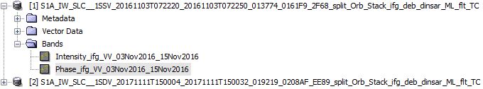
Once done, you will get two data for each earthquake example, like this
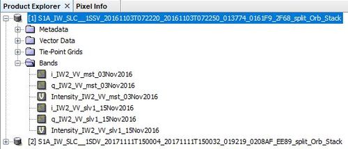
[1] is 2016 Kaikoura earthquake;[2] is 2017 Iran–Iraq earthquake

The file suffix will be: _split_Orb_Stack

Step5: Interferogram Formation

This step computes the phase difference map and attempts to eliminate other sources of error such as the curvature of the reference surface.
The interferometric fringes form where there is interference between the two signals. Fringes are represented by a 2π (360 degree) cycle with each colour depicting a particular range of this cycle. Denser fringes represent greater change between the two images.

Go to find Radar -> Interferometric -> Products -> Interferogram Formation

Select both coregistered files respectively and click Run with default settings

The file suffix will be: _split_Orb_Stack_ifg
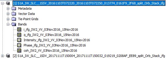
[1] is 2016 Kaikoura earthquake; [2] is 2017 Iran–Iraq earthquake

You can preview the phase map by clicking Phase_ifg_ in Band
Here is a preview of Phase map for the 2016 Kaikoura earthquake (Top) and 2017 Iran–Iraq earthquake (bottom): :

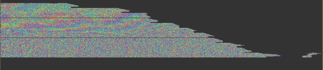
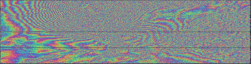
[NOTE: This is not the final output of interferogram !!]

Step6: Deburst

This step is to join each burst we selected in a single image

Go to find Radar -> Sentinel-1 TOPS -> S1 TOPS Deburst
Select file for each example, click Run with default settings
The file suffix will be:_split_Orb_Stack_ifg_deb
[1] is 2016 Kaikoura earthquake; [2] is 2017 Iran–Iraq earthquake

Step7: Topographic Phase Removal

This step removes known topographic phase contributions using a reference DEM. This emphasizes the phase changes related to the deformation.

Go to find Radar -> Interferometric -> Products -> Topographic Phase Removal

Select interferogram file for each example and click Run with default settings
The file suffix will be:_split_Orb_Stack_ifg_deb_dinsar
[1] is 2016 Kaikoura earthquake; [2] is 2017 Iran–Iraq earthquake

Step8: Multi-looking

Multi-looking is a common filtering technique used to increase the signal-to-noise ratio of the resulting image.

Go to find Radar -> SAR Utilities -> Multilooking

Select source for each example
Click Processing Parameters select two source bands as above shows
- Click Run with default settings
The file suffix will be: _split_Orb_Stack_ifg_deb_dinsar_ML
[1] is 2016 Kaikoura earthquake; [2] is 2017 Iran–Iraq earthquake

Step9: Phase Filtering

Goldstein Phase-filtering is another technique used to increase the signal-to-noise ratio. It is considered to be a state-of-the-art technique and will drastically improve the interferometric phase map such that the ring patterns associated with ring-patterns will be clearly visible.

Go to find Radar -> Interferometric -> Filtering -> Goldstein Phase Filtering

Select source product for each example
Click Run with default settings
The file suffix will be: _split_Orb_Stack_ifg_deb_dinsar_ML_flt

[1] is 2016 Kaikoura earthquake; [2] is 2017 Iran–Iraq earthquake
You can preview the phase map by clicking Phase_ifg_ in Band
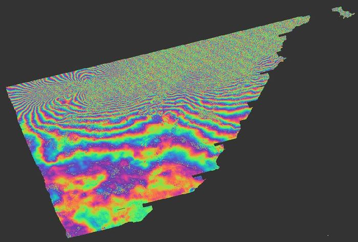
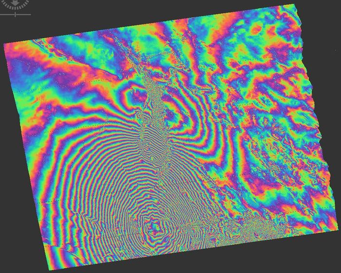
Here is exampled preview of Phase map of 2016 Kaikoura earthquake (Top) and 2017 Iran–Iraq earthquake (bottom):

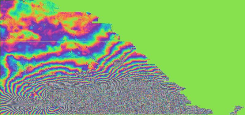
[NOTE: We got the final output of interferogram !! but still need a bit more steps.]

Step10: Geometric Correction

For the interferogram to be useful, it needs to be projected onto a geographic coordinate system using a reference DEM. This step should only be done once all processing on the image completed and the image is ready to be exported.

Go to find Radar -> Geometric -> Terrain Correction -> Range-Doppler Terrain Correction
Click Processing Parameters select phase source bands for each example as above shows
- Click Run with default settings
The file suffix will be: _split_Orb_Stack_ifg_deb_dinsar_ML_flt_TC
[1] is 2016 Kaikoura earthquake; [2] is 2017 Iran–Iraq earthquake
You can preview the phase map by clicking Phase_ifg_ in Band
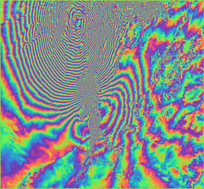
Here is exampled preview of Phase map of 2016 Kaikoura earthquake (Top) and 2017 Iran–Iraq earthquake (bottom):

Step11: Export Data

To export data so that you can use the output in other GIS or geospatial software, there are many file types that you convert into.
So in this example, we will convert these outputs into Google Earth so that you can view the earthquake deformation in actual earth surface.

Go to find File -> Export -> Other -> View as Google Earth KMZ
The file will be like:
[1] is 2016 Kaikoura earthquake; [2] is 2017 Iran–Iraq earthquake

[NOTE : To convert into KMZ must be geocoded (step10) !! ]

Results

Now, after you import them into Google Earth or any other software, you can view the interferogram of earthquake deformation for two examples.
The coloured fringes indicate that the deformation of the earth surface is around 2.8 cm between each colour cycle.

Earthquake magnitude distribution of 2016 Kaikoura earthquake

Earthquake magnitude distribution of 2017 Iran–Iraq earthquake

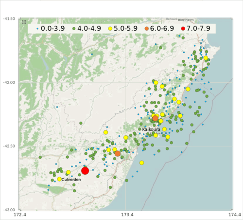
Compare to the Earthquake magnitude distribution map on the right for both examples, the epicentre is basically corresponding to the central fringe at interferogram, which will help to detect surface deformation after earthquake.

Automating the Process (Advanced)

For this section you will need Python installed on your machine. It is recommended to install Python through Anaconda; however this is not a necessity if you are familiar with installing and configuring Python libraries. The following link provides access to a GitHub repository containing a Python script that automates the process described in this tutorial. The script uses the SNAP Python API, snappy.

Creating Interferograms using Snappy

The repository contains a .yml file that can be used to set up a conda environment and also includes instructions on how to configure snappy for this environment (if you are running Windows 10). As previously stated, these steps are not necessary if you are comfortable with installing and configuring Python libraries. Instructions on downloading and configuring snappy can be found here.

References

The European Space Agency. (2012). Sentinel-1. Retrieved 2 December 2019.

Veci, L. (2014). Sentinel-1 Toolbox - Interferometry Tutorial. Retrieved 2 December 2019.

User Guides - Sentinel-1 SAR - Interferometry. Sentinel Online. European Space Agency. Retrieved 2 December 2019.

Podest, E.(2017). Generation of an Interferogram – Earthquake Deformation. Retrieved 2 December 2019.