Creating a 3d Model for a Ski Hill in Aspen using QGIS
Contents
Introduction and Purpose
This tutorial will demonstrate how QGIS can be used to create a 3D model and how to effectively create a model that will best represent what the user is trying to achieve. This tutorial shows how creating 3D models can be more effective than a 2D map for certain situations where elevation change and reference is important. To demonstrate, this tutorial will generate a 3D model of Aspen Snowmass Ski Resort, near Aspen, Colorado. You will create ski runs, gondola routes, and the 3D terrain which allow for an effective visualization. This tutorial is meant for users who are new to 3D modelling but are also relatively experienced with QGIS and the main functions.
To get started, ensure you have the latest version of QGIS downloaded, the latest stable release at the time of writing is 3.40.11 Bratislava.
It is also recommended that this tutorial be completed on a computer with significant graphics processing power, as the manipulation of the DEMs and 3D visuals can be demanding.
Downloading Imagery from Earth Explorer
In order to create a 3D model, we need elevation data. This elevation data will be the key to accurate 3D representation of your chosen terrain.
The elevation data which we will use for this model is accessed through the United States Geological Survey's Earth Explorer portal, which can be accessed using this link: https://earthexplorer.usgs.gov/ A USGS account is required in order to download the data, however the process is quick and an account is free for educational purposes.
This tutorial will use the Aspen Snowmass ski resort as a focus area, so we need to find Aspen in the USGS map pane.

Once you have located Aspen on the map, we will create a study area using the "Polygon" feature in the left menu pane. You can input manual coordinates, however the "Use Map" function is much more intuitive and makes defining our search area easier. By clicking "Use Map", the coordinates of your current map extent will automatically be set as the search bounds, so ensure Aspen and the Snowmass Village to the West are within your map pane.

Once your search area has been defined on the map, select "Data Sets" from the bottom left search pane. One option to complete this tutorial is Landsat 2 Imagery DEM. Another popular DEM dataset is the Shuttle Radar Topography Mission data, which can be found under Digital Elevation > SRTM. Some benefits of the SRTM data is the greater worldwide coverage available through USGS, as well as the smaller footprint of each DEM, which reduces file size of the GeoTIFF. Once you have decided which data you would like to work with, select "Results". This will return a list of datasets from your chosen collection, which encompass the study area you defined in the Search Criteria.


To ensure the returned datasets properly cover the area you wish to work with, check the footprint of the imagery by clicking the foot icon in the results list. This will show a polygon representing the geographic extent of the data.

If the returned dataset looks to cover the area you will be working on, click the Download Options button on the same list as the footprint.

From the pop-up download menu, choose the GeoTIFF 1 Arc-second option. Your data should begin downloading immediately.
Creating your Study Area
Once the data is downloaded, you can now input the dataset into a QGIS project. As you can see, your data covers a large area, most of which we will not use in our model of the ski hill. It would be best to clip this image to a smaller extent near the ski hill in Aspen, and not include the other areas. In order to do this, we first need a base map so that we can see the ski mountains in the area. One of the easiest ways to do this is through the HCMGIS plugin.

Downloading this plugin will add a "HCMGIS" menu to the QGIS toolbar. From here, you can quickly add a selection of basemaps to your project, either raster or vector, from a variety of different sources. For now, choose the "Google Satellite Hybrid" basemap, so we can locate the study area.

This will show Google Earth with Google Maps as well so you can find your ski mountain. Once you have found the Aspen Snowmass Ski Resort, double check that it is within the extent of your DEM data. Once this is confirmed, create a polygon layer around the ski hill. After the polygon is created, Use the "Clip Raster by Extent" tool to clip the DEM to the polygon that you created so that the DEM is only the size of the ski hill. This will limit the extent of your study area, and ensure the ski hill of interest is the focal point of your 3D model. Ensure you set a file path for your clipped raster to be saved as a permanent file.

Creating your Map
There are two final steps to complete before we can begin our 3D model. First, we will install the QuickOSM plugin into QGIS, in order to easily extract data for the ski trails and lifts on Snowmass Mountain.

Once installed, open the QuickOSM plugin, and navigate to the Quick Query menu. Enter piste:type in the key column, and downhill in the Value column of the first row. It is usually easiest to set the data extraction extent to your Canvas Extent, as this will only download OpenStreetMap data that meets the criteria within your current map pane (which should still be focused on the Snowmass Resort).
.png)
Run a second Quick Query in the QuickOSM plugin, this time with aerialway in the key column, and leave the value column blank in order to query all values within. Both the ski trails and lift data can be extracted in one query, however in this case it is helpful to have them in separate packages to facilitate manipulation of symbology and rendering.
Before we move on, it would be best to fix up the symbology of your ski trails and lifts. Some things to keep in mind while designing your symbology:
- Ski run colour indicates difficulty, a categorized symbology works best here:
- Green - Easy
- Blue - Intermediate
- Black - Expert
- White text with a thin black buffer is often easiest to read over a varied background.
- Labels indicating trail names can become crowded with so many separate routes - consider whether they're needed at all for your use.
The second and final step before we create the 3D model is to add a connection to the ESRI ArcGIS World Imagery Server. This will provide us convenient access to high resolution imagery which is often superior to that offered by the Google Maps Satellite base map.
In the browser pane in QGIS, locate the ArcGIS REST Servers item, right click and select New Connection. This will open the connection window where you must input a name, and provide the following URL:
https://services.arcgisonline.com/ArcGIS/rest/services/World_Imagery/MapServer
With these two boxes filled out, select OK to establish the connection. Successfully completing this process should provide you with a wide selection of metadata and imagery at different resolutions to add directly into your QGIS projects. For our model, drag the High Resolution 30cm Imagery raster data into the project.
Creating your 3D Model
After georeferencing everything you need, you can now start to work on the 3D model. There are crucial steps that have to be taken to create a 3D model that looks good.
1. Download the Qgis2threejs plugin.

2. Everything set to visible in your QGIS project window will be rendered on your 3D model, so ensure your symbology, rendering order, etc. is set as you wish it to be in the final product.
3. Open Qgis2threejs, to do this click "Web" then click "Qgis2threejs" and select "Qgis2threejs Exporter".

4. Now, it is time to add your map to Qgis2threejs. To do this, click the checkmark for the DEM you wish to use. This will add the DEM with all the ski and gondola routes created.

5. You will notice something wrong with the image, this is because the DEM is not clipped with the polygon. Even though you already did this, the plugin does not recognize it. To fix this, right-click the DEM and select properties. Once this is selected, select the checkbox next to "Clip DEM with polygon layer".


6. Now that everything is clipped properly with the 3D image, it is time to enhance the image to make it look better. You may notice that there is not actually a lot of elevation for your image. This can be changed in the "Scene Settings". To get there, select "Scene" in the top left section, then select "Scene Settings". This will bring up a menu, in this menu you can change the Z exaggeration. This will change how intense the elevation change is represented in your model. Exaggeration in the range of 2-4 usually provide the best results for a study area of this size. It brings out enough elevation to properly evaluate the ski runs on the map, with minimum distortion to the imagery layer.


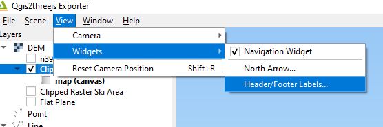
7. Adding a north arrow is the next step. To add the north arrow, click "View", then "Widgets", then "North Arrow". Once this is completed, a north arrow should appear on the bottom left of the screen.
8. Now that the north arrow is on the 3D model, the next step is to add a legend. This step is fairly different than when regularly using QGIS. First, set your project layers into the proper order in your QGIS project window (not the Qgis2threejs plugin). Return to Qgis2threejs, click "View", then "Widgets", then "Header/Footer Labels". Once this is selected, you will be brought to a screen that gives you the option to either type in a header or a footer. In the header section, type: <img src="legend.png" alt="Legend">. This will add a little box with a question mark at the top left of the screen. The only way the legend is going to appear, is if your PNG legend image is saved to where you are going to export your 3D model.

Your 3D model should look like these images so far:


Uploading your 3D Model
Once your 3D model is created, your legend is ready, and the north arrow is working. It is time to upload the 3D model. In order to do this:
1. Select "File"
2. Select "Export to Web"
3. Set the output directory to the location where you want your model saved.
4. Practice good naming conventions and set the HTML filename to something descriptive of the 3D model.
5. Make sure to select "Enable the viewer to run locally". If you do not select this, you will not be able to view your 3D model.
6. Now select "Export"
7. Your 3D model should be created!
Here is what your 3D model should look like once it is uploaded as an HTML file:


Conclusion
The purpose of this tutorial was to demonstrate the advantages of using 3D maps in scenarios involving elevation data. When comparing the 3D model to the corresponding 2D map, it's clear that the 3D visualization makes it much easier to trace the ski routes, and evaluate their vertical intensity. Navigating with the 2D map can be challenging, especially when trying to determine the next path to follow. In contrast, the 3D map offers clearer guidance, making it simpler to move from one ski route to the next.
References
N/A(2023) Earth Explorer, https://earthexplorer.usgs.gov/ (Accessed: 20 December 2023).
Llaves (2018) Legend for 3D Maps · issue #121 · Minorua/qgis2threejs, GitHub. Available at: https://github.com/minorua/Qgis2threejs/issues/121 (Accessed: 20 December 2023).