Creating as Site Suitability Map for Emergency Services using QGIS

Author: Harith T Harison Course: GEOM 4008 – Open Source Geospatial Systems Semester: Fall 2025

Overview

This tutorial demonstrates how to use open data and the open-source GIS software QGIS to identify underserved areas for emergency services (e.g., fire, police, ambulance) and propose new facility locations in the City of Ottawa. The workflow uses only freely available datasets and tools and can be replicated by anyone with access to QGIS. For this particular tutorial we will be focusing on fire stations in Ottawa. I will also add additional material and shapefiles to experiment with using the same process.

The analysis focuses on:

• Mapping existing emergency service coverage
• Overlaying population distribution
• Identifying areas that fall outside of current service buffers
• Proposing candidate locations for new facilities
• (Optional) Automating key steps using the QGIS Graphical Modeler

The methods shown here can be adapted to other cities, services, or types of public facilities.

Learning Objectives

By the end of this tutorial, you will be able to:

1. Download and prepare open geospatial datasets for a local suitability analysis.
2. Set up a QGIS project with an appropriate projected coordinate reference system.
3. Map current emergency service coverage using buffer analysis.
4. Combine population data with service coverage to identify underserved areas.
5. Digitize and evaluate candidate locations for new facilities.
6. Create a cartographic map layout suitable for reporting or presentations.
7. (Optional) Build a simple automated workflow using the QGIS Graphical Modeler.

Software and Data Requirements

Software

You will need:

• QGIS 3.x (any recent long-term release is recommended)
• Internet access to download open data

No proprietary software (e.g., ArcGIS) is required for this tutorial.

Data Sources

You will need to obtain the following open datasets (or similar equivalents):

• Ward or municipal boundary for Ottawa

 * Source: City of Ottawa Open Data Portal (“Municipal Wards”)

• Existing emergency service facilities

 * Source: City of Ottawa Open Data Portal (“Fire Stations”, “Police Stations”, “Paramedic Posts” or combined “City Facilities” dataset)

• Road network

 * Source: City of Ottawa Open Data Portal (“Road Centreline”) or OpenStreetMap

• Population data

 * Source: Statistics Canada (census polygons with population counts) or City of Ottawa ward/DA-level population

• (Optional) Neighbourhood equity or vulnerability index

 * If available as open data, this can be used as an additional criterion.

• Optional
  • You can download Data sets like current Libraries/Museums from the portal and also use those for site suitability.

Study Area

This tutorial focuses on the City of Ottawa, with special attention to an example ward (e.g., Ward 19). However, the steps can be applied to any ward or neighbourhood. If you are using a different study area, substitute your own boundary layer where “Ward 19” is mentioned. A different ward could be selected depending on your preference or your choice of logic.

Part 1 – Set Up Your QGIS Project

1. Open QGIS.
2. Go to Project → New.
3. Set the project coordinate reference system (CRS):
   1. In the bottom-right corner of QGIS, click the CRS indicator.
   2. Search for and select: EPSG:26918 – NAD83 / UTM Zone 18N.
   3. Click OK.
4. Save the project:
   1. Go to Project → Save As…
   2. Choose a location and name the project file, e.g., `Emergency_Services_Ottawa.qgz`.

Part 2 – Download and Load the Data

2.1 Download data from open portals

Using your web browser:

1. Go to the City of Ottawa Open Data Portal.
2. Download:
   1. Ward or municipal boundary layer (e.g., Shapefile or GeoJSON)
   2. Emergency service facility layer(s) (fire, police, paramedic, etc.)
   3. Road centreline layer
3. Go to Statistics Canada or another open data portal and download:
   1. Population polygons (e.g., dissemination areas, census tracts, or wards) with a population attribute.
   2. You can use this link to find the required Open Data Layers required for this tutorial: https://open.ottawa.ca/

Extract any ZIP files to a working folder on your computer.

2.2 Load data into QGIS

1. In QGIS, go to Layer → Add Layer → Add Vector Layer….
2. Browse to your ward boundary file and click Add.
3. Repeat for:
   1. Emergency facilities
   2. Road network
   3. Population polygons
4. Confirm that all layers appear in the Layers Panel and are visible on the map.

1. 1. [Layers SS]

Part 3 – Reproject Layers to a Common CRS

Even if layers appear together, they may use different CRSs. It is good practice to work in a uniform projected CRS.

For each layer:

1. Right-click the layer → Properties → Source. Note the layer’s CRS.
2. If any layer is not in EPSG:26918:
   1. Open the Processing Toolbox: Processing → Toolbox.
   2. Search for and run “Reproject layer” (Vector general).
   3. Set:
      1. Input layer: your original layer
      2. Target CRS: EPSG:26918 – NAD83 / UTM Zone 18N
      3. Save the output as a new file with “_utm18” in the name.
   4. Click Run.

1. 1. insert Source and Project Coordinates here

After reprojecting all layers:

1. Remove the original versions (if desired) and keep only the “*_utm18” versions.
2. Ensure your project CRS remains EPSG:26918.

Part 4 – Define the Study Area (Ward Subset)

4.1 Visualize population density

If your population layer does not already have a population density field, you can create one by dividing population by area. In our Data we don't have an Area section and we will be sorting out by Population alone.

Optional( If you have Area on your attribute table)

1. Right-click the population layer → Open Attribute Table.
2. Click Field Calculator.
3. Create a new field, e.g., `pop_dens`, and choose a suitable numeric type (e.g., Decimal).
4. Expression example:

 `"POPULATION" / $area`
 (Adjust `"POPULATION"` to your actual population field.)

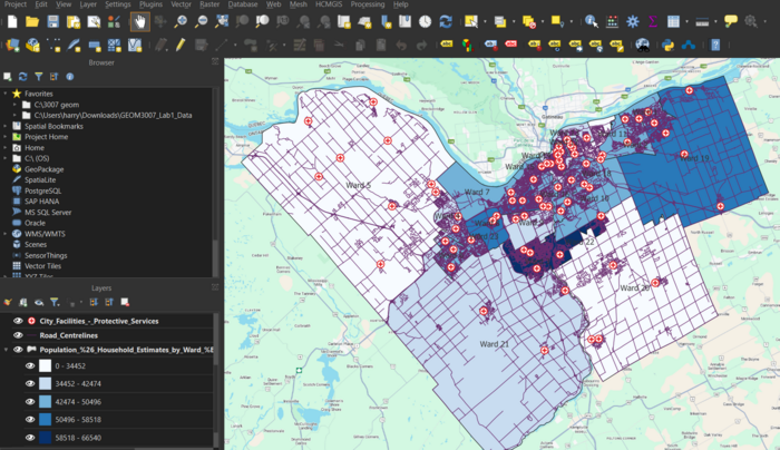
Apply graduated symbology:

1. Right-click population layer → Properties → Symbology.
2. Change type to Graduated.
3. Column: select `pop_dens` (or your density field) / select 'POPULATION'.
4. Choose 5 classes and a suitable colour ramp (e.g., light to dark).
5. Click OK.

In this example, we focus on a single ward, such as Ward 19. Since visually from the chorolopleth layer we can see that there is high population wards 21 and 19 but few fire stations.

1. Open the attribute table of your ward boundary layer:
   1. Right-click ward layer → Open Attribute Table.
2. Click the “Select features using an expression” icon.
3. Use an expression similar to:

 `"WARD_NAME" = 'Ward 19'`
 (Adjust the field and ward name to match your dataset.)

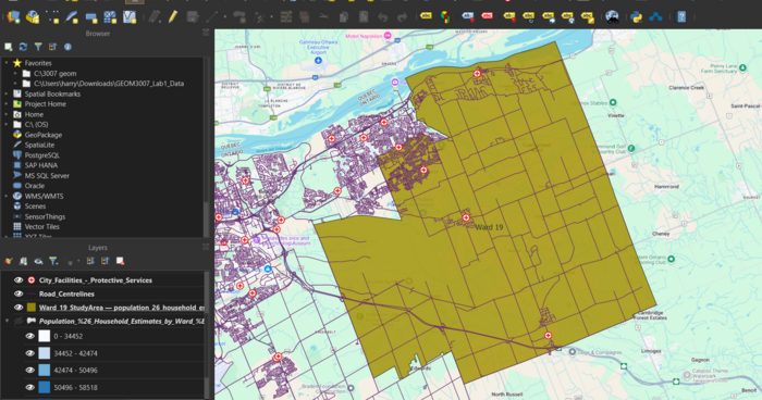
1. Once Ward 19 is selected, right-click the ward layer → Export → Save Selected Features As….
2. Save as a new layer, e.g., `Ward19_StudyArea`.
3. Add the new layer to the map if it does not appear automatically.

[Insert screenshot: Ward 19 selected and saved as separate layer]

Optional: You can make your study area smaller by digitizing a custom polygon for only the southern portion of the ward.

Part 5 – Map Current Emergency Service Coverage

5.1 Clip facilities and roads to the study area

1. Open the Processing Toolbox.
2. Search for “Clip” (Vector overlay → Clip).
3. Set:
   1. Input layer: emergency facilities layer (reprojected)
   2. Overlay layer: `Ward19_StudyArea`
   3. Output: `Facilities_Ward21`
4. Click Run.
5. Repeat the process for the road network, saving as `Roads_Ward21`.

5.2 Create buffers around existing facilities

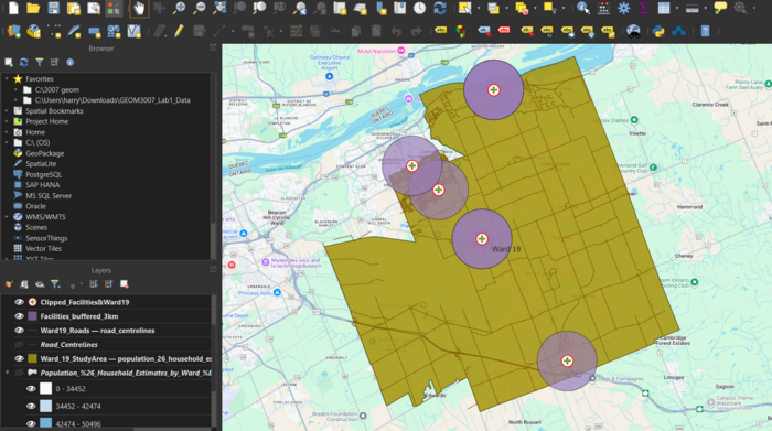
We will assume a 3 km service radius as an example. You can adjust this based on realistic response distances.

1. In the Processing Toolbox, search for “Buffer” (Vector geometry → Buffer).
2. Set:
   1. Input layer: `Facilities_Ward19`
   2. Distance: 3000 (for 3,000 meters)
   3. Segments: 20 (default is fine)
   4. Dissolve result: choose either ON or OFF depending on whether you want merged coverage.
   5. Output: `Facilities_Buffer_3km`
3. Click Run.

Style the buffer layer:

1. Right-click `Facilities_Buffer_3km` → Properties → Symbology.
2. Choose a light fill colour with transparency so underlying layers remain visible.

[Insert screenshot: Map showing buffers over population density]

Part 6 – Identify Underserved Areas

We now identify areas inside the ward that fall outside existing service buffers.

6.1 Compute “unserved” area

1. In the Processing Toolbox, search for “Difference” (Vector overlay → Difference).
2. Set:
   1. Input layer: `Ward19_StudyArea`
   2. Overlay layer: `Facilities_Buffer_3km`
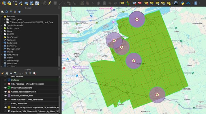
   3. Output: `Unserved_Area_Ward19`
3. Click Run.

The resulting layer represents areas within the ward that are not within 3 km of an existing facility.

6.2 Combine unserved areas with population data

If your population units are smaller polygons (e.g., census tracts or DAs), you can intersect them with the unserved area to locate high-population unserved zones.

1. OPTIONAL
2. In the Processing Toolbox, search for “Intersection”.
3. Set:
   1. Input layer: population polygons
   2. Overlay layer: `Unserved_Area_Ward19`
   3. Output: `Unserved_PopBlocks`
4. Click Run.

Open the attribute table of `Unserved_PopBlocks` and sort by population or density to see which unserved polygons have the highest demand.

[Insert screenshot: Unserved areas with population polygons]

Part 7 – Propose Candidate Locations for New Facilities

There are many ways to choose new sites. In this tutorial, we will manually place candidate points in high-population unserved areas near major roads.

7.1 Create a new point layer for candidate facilities

1. Go to Layer → Create Layer → New Shapefile Layer….
2. Set:
   1. Geometry type: Point
   2. CRS: EPSG:26918 – NAD83 / UTM Zone 18N
3. Add fields such as:
   1. `id` (Integer)
   2. `type` (Text, e.g., “Fire”, “Police”, “Ambulance”)
4. Click OK and save as `Proposed_Facilities`.

7.2 Digitize new facility locations

1. Ensure `Proposed_Facilities` is selected in the Layers Panel.
2. Toggle editing: right-click the layer → Toggle Editing, or click the pencil icon.
3. Use the Add Point Feature tool to click on map locations within:
   1. High-population unserved areas, and
   2. Close to main roads from `Roads_Ward19`.
4. For each point, enter `id` and `type` attributes.
5. When finished, click Toggle Editing again and save edits.

7.3 Buffer new facilities

1. Run the Buffer tool again:
   1. Input layer: `Proposed_Facilities`
   2. Distance: 3000 (or another chosen radius)
   3. Output: `ProposedFacilities_Buffer_3km`
2. Click Run.

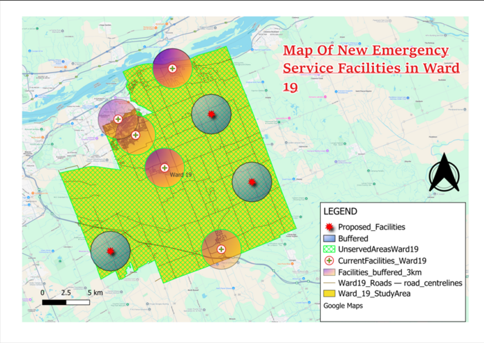
You now have a map showing both the existing and proposed coverage.

Part 8 – Create a Final Map Layout

1. Go to Project → New Print Layout….
2. Give the layout a name, e.g., `Emergency_Services_Final_Map`.
3. In the Layout window, click Add Map and drag a rectangle where the map should go.
4. Adjust the map’s extent using the navigation tools so that your study area and buffers are clearly visible.
5. Add map elements:
   1. Add Legend – customize layer names to be understandable (e.g., “Existing Facilities”, “Proposed Facilities”, “3 km Coverage”, “Population Density”).
   2. Add Scale Bar
   3. Add North Arrow
   4. Add Label for title, e.g., “New Locations for Emergency Services in Ottawa”.
6. When satisfied, export the layout:
   1. Layout → Export as PDF or Export as Image.

[Insert screenshot: Final layout with legend, scale bar, and title]

Conclusion

This tutorial demonstrated how open data and open-source GIS tools can be used together to support data driven decision making for public service planning. By combining population density, existing facility locations, and service coverage buffers, we identified areas within Ottawa specifically parts of Ward 19 that are underserved by current emergency services. QGIS provided all the tools needed to complete this workflow, from data preparation to analysis and cartographic output, proving that complex spatial suitability studies can be carried out fully within a free and accessible software environment. The methods shown here are easily adaptable to other cities, facility types, or datasets, making this workflow a flexible starting point for more advanced planning, modeling, or community-focused analyses

Part 9 – (Optional) Automate the Workflow with QGIS Graphical Modeler

This optional section shows how to automate key steps (clip → buffer → difference → intersection) so that the process can be rerun with different input layers or parameters.

9.1 Open Graphical Modeler

1. Go to Processing → Graphical Modeler….
2. Click New Model.
3. Set:
   1. Model name: `Emergency_Service_Suitability`
   2. Group: e.g., `EmergencyPlanning`

9.2 Add model inputs

On the left panel:

1. Under Inputs, drag and drop:
   1. Vector Layer – name it “Study area”
   2. Vector Layer – name it “Existing facilities”
   3. (Optional) Vector Layer – name it “Population polygons”
   4. Number – name it “Buffer distance (m)” and set a default (e.g., 3000)

9.3 Add algorithms

1. Add Clip:
   1. Double-click Clip (Vector overlay).
   2. Set:
      1. Input layer: “Existing facilities”
      2. Overlay layer: “Study area”
      3. Output: “Facilities in study area”
2. Add Buffer:
   1. Input layer: “Facilities in study area”
   2. Distance: “Buffer distance (m)”
   3. Output: “Existing coverage buffer”
3. Add Difference:
   1. Input layer: “Study area”
   2. Overlay layer: “Existing coverage buffer”
   3. Output: “Unserved area”
4. (Optional) Add Intersection with population:
   1. Input layer: “Population polygons”
   2. Overlay layer: “Unserved area”
   3. Output: “Unserved population blocks”

Mark the final outputs (e.g., “Unserved area”, “Unserved population blocks”) as model outputs.

9.4 Save and run the model

1. Click Save and close the model editor.
2. In the Processing Toolbox, expand Models - EmergencyPlanning (or your chosen group).
3. Double-click `Emergency_Service_Suitability`.
4. Choose your study area, existing facilities layer, population layer, and buffer distance.
5. Click Run.

The model will automatically create the unserved area and (optionally) unserved population blocks, simplifying repeated analyses or applications to other wards or cities.

Troubleshooting Tips

• If layers do not align, check that all are reprojected to the same CRS (EPSG:26918).
• If the Difference or Intersection tools give empty outputs:
  • Confirm that the input layers indeed overlap spatially.
  • Check for invalid geometries (use Vector - Geometry - Check validity).
• If your map looks cluttered, simplify symbology:
  • Use subtle fills for buffers and stronger symbols only for proposed sites.
  • Turn off labels for layers that are not essential to the final map.
• If buffering shows and error where distance isn't shown in units
  • Make sure new layer has same projections or switch it in 'Properties' - 'Source'.

Data Sources and Licensing

• City of Ottawa Open Data Portal – municipal boundaries, facilities, and roads
• Statistics Canada – census polygons and population counts
• OpenStreetMap – additional road and facility information

All datasets used in this tutorial should be under open licenses that allow reuse and redistribution.