Determining Effects on Temperature Interpolations from Large Lakes using QGIS
Contents
Introduction
Purpose
The purpose of this tutorial is to provide a guide for creating an Inverse Distance Weighting (IDW) interpolation in GRASS GIS, and analyzing the spatial errors produced in interpolated data by large interrupting features. This tutorial will aim to create a usable set of layers in QGIS, including an Ontario shapefile, an Ontario lakes shapefile, and a point vector layer of temperature data collected at climate stations in Ontario. Next, the guide will demonstrate how to use these layers to create an IDW interpolated raster layer for temperature using GRASS GIS. Finally, the guide will instruct the user to create a graph in R in order to analyse the errors produced in the interpolation.
Background Information
An Inverse Distance Weighted (IDW) interpolation follows Tobler's First Law of Geography; near things are more alike than things that are farther apart. IDW uses the values surrounding the location of interpolation to a certain distance and assigns weighting factors to them. Values that are closer to the area being predicted have more weight in predicting the value than values that are further away. IDW interpolation is sensitive to outliers.
In Canada, the Great Lakes are key geographic features whose effects are as strong as to create a weather phenomenon that impacts the temperature of neighboring land regions. The concept of lake-effect is that large bodies of water are slow to react to changes in temperature; they stay warmer for longer in the winter than the temperature on land, and they remain cold well into the spring. For this reason, locations that border large lakes, such as the Great Lakes and the world oceans, have their temperature moderated by the movement of warm or cool air off of the bodies of water. Lake-effect also causes variations in moisture over nearby land masses leading to coastal weather being very unique.
This effect can cause and propagate errors in interpolations due to the nature of the phenomenon.
This project has additional uses outside of lake-effect as well, as you could analyze errors in temperature interpolation caused by urban heat islands, or errors in interpolation caused by other types of large geographic features that relate to geospatial phenomenon like weather.
Software
The software used for this project was QGIS, GRASS GIS, and R, which are free and open-sourced GIS and statistical software.
The software can be downloaded here: https://www.qgis.org/en/site/forusers/download.html for QGIS and https://grass.osgeo.org/download/ for GRASS GIS. R can be downloaded from https://www.r-project.org/.
QGIS was used to set up the data into a usable form (i.e. correct projection). GRASS GIS was then used to create the interpolation and data extraction for further interpretation. R was used to analyze the data and examine the spatial error in a graph.
Data
The data used in this tutorial includes a shapefile of Ontario, a shapefile of lakes within Ontario, and temperature data for climate stations in Ontario represented as points. In this tutorial there will be two examples completed; one using data from a date in spring (the area beside the lake should be cooler than everywhere else) and one using data from a date in late fall (the area beside the lake should be warmer than everywhere else).
The data can be found and downloaded at the following links: Ontario boundary file: https://www.dropbox.com/s/zhun4vrudwiww0y/Ontario.gpkg?dl=0 Ontario lakes file: https://www.dropbox.com/s/rbjwwgs22qc17ih/Ontario_lakes.gpkg?dl=0 Climate data for Ontario: https://climate.weather.gc.ca/prods_servs/cdn_climate_summary_e.html
To download climate data; select a date of interest and the province of interest and download data as a .csv.
This tutorial will work for any point values for the interpolation.
Tutorial
Loading the Data in QGIS
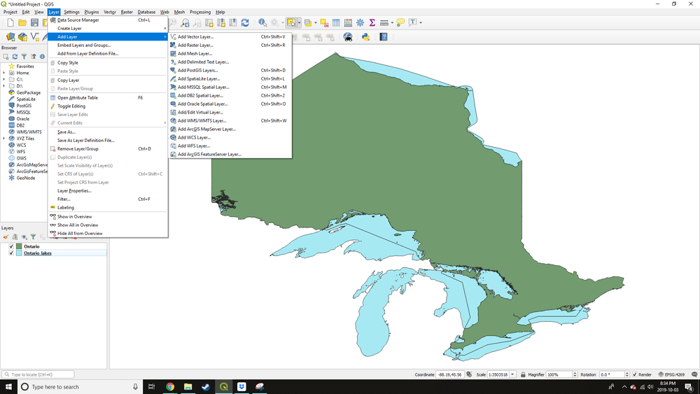
After installing the software and downloading the data, the first step is to open up the layers in QGIS. Use Add Vector Layer, as the Ontario and Ontario_lakes files are in vector format. See the image below to navigate to this step.
Figure 1. Layer > Add Layer > Add Vector Layer
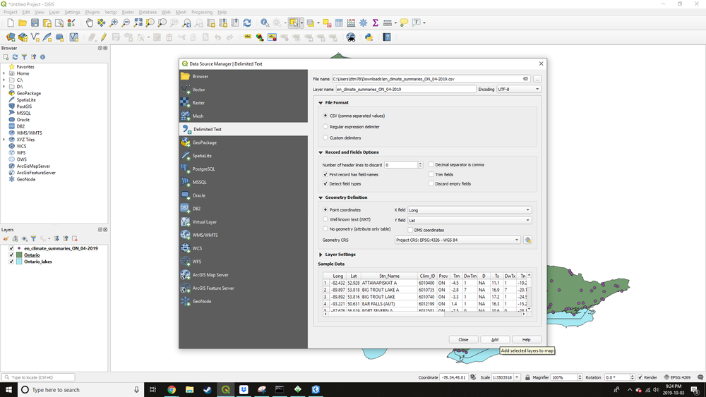
To add the temperature point data use Add Delimited Text Layer instead of Add Vector Layer. Add the file from your data, and select CSV for the file format (Note: Make sure the table file is set as CSV). For this file, there should be no header checked, and fields 3 and 4 are used for X field and Y field respectively. See the image below to navigate to this step.
Figure 2. Adding the climate data, which is a delimited text layer, and adjusting the options in the window.
Setting up Validation and Training Data in GRASS GIS
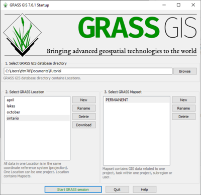
Now that the data are imported and in the proper format, we can add them to GRASS GIS for the IDW interpolation. When opening GRASS an opening screen pops up which helps to set up the database that the project will be located in. Using this screen, create a directory and new location with an appropriate project name. The mapset will auto-generate a "PERMANENT" project folder that only the creator can add data to. Proceed to start GRASS GIS.
Figure 3. The opening screen for GRASS GIS. This series of menus aids the user in setting up the location for the project.
In order to upload all of the data to the new project, data must be added according to data type. The Ontario file and Ontario_lakes file can both be added using File > Import vector data > Simplified vector import with reprojection.
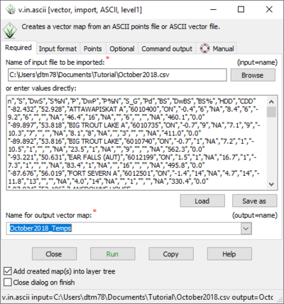
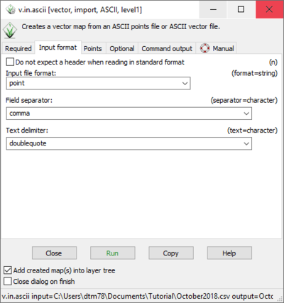
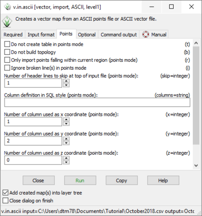
The .csv file containing the temperature data must be added using File > Import vector data > ASCII points or GRASS ASCII format. In the window that opens up
Figure 4. On the Required tab in the ASCII window, ensure that the correct input file is selected then load the values and name the output file.
Figure 5. On the Input format tab in the ASCII window, ensure that the file format, field separator, and text delimiter as as shown.
Figure 6. On the Points tab in the ASCII window, ensure that the number of header lines to skip is correct, in this case 1, and that the x and y coordinates match up to the correct columns in the .csv.
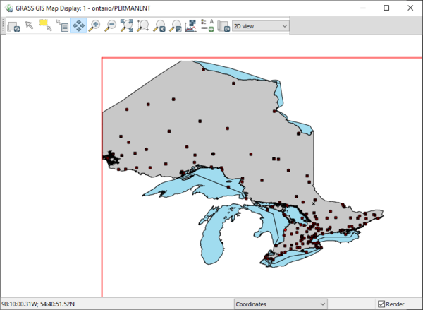
Once the data is properly uploaded the layers should be visible on the map display.
Figure 7. Map view in GRASS GIS. All layers should be visible. Symbology can be manipulated using the button to the right of the layer names in the display list (located in the other window).
Firstly, the temperature data should be separated into validation and training sections to use. This is done using Vector > Feature Selection > Select by Attributes.
In this tutorial, we'll use 20% of the points for validation, and 80% of the points for training. Select the temperature file for input and name your output points. Ensure you name the output file appropriately so that the validation and training data are distinct.
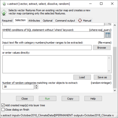
On the next tab (Selection), scroll to the bottom and put the appropriate number for 20% of the points in the box. For this tutorial there were 187 climate stations, so 20% of the points was about 38 points.
Figure 8. In the Select by Attribute window on the Selection tab, mark down approximately 20% of the data points for validation.
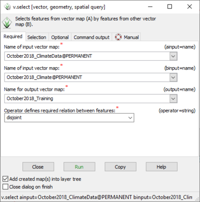
Next, the training points can be selected using Vector > Feature Selection > Select by Another Map. Use your temperature file for the first input (ainput), your validation file for the second input (binput), name the output, and select "Disjoint" for the operator. This will create a new file for the training points.
Figure 9. In the Select by Another Map window ensure the operator is set to "Disjoint".
IDW Interpolation in GRASS GIS
The interpolation can now be executed using Raster > Interpolate Surfaces > IDW from Vector Points. The input vector map should be the training data, and the output should be named as the IDW interpolation. In the Values tab the name should reference the column with the temperature values, so the column name is Pd in this example. The remaining fields can be left at default, and the interpolation can be run.
Figure 10. The completed interpolation for the October temperature data in Map View.
Figure 11. The completed interpolation for the April temperature data in Map View.
Cross-Validation of the Interpolation in GRASS GIS
You can now use the validation points to cross-validate the IDW interpolation. This can be done using Vector > Update Attributes > Sample Raster Neighbourhood Around Points. Select the validation points as the input, the temperature data for the column, the IDW for the raster, and name the output file appropriately.
Next, the distance from each point to the nearest lake should be known. This can be found using Vector > Nearest Features. Select the validation points as the input on the From tab, and the Ontario_lake file for the input on the To tab.
The data can now be extracted to a .csv to be used for analysis via File > Export Database Table > Common Formats Using OGR. Use the output from the Nearest Feature process as the input and dsn, and choose the Table format to be a .csv.
Statistical Analysis in R
The resulting CSV can now be analyzed using a variety of programs (R, excel, etc.) that can create graphs and figures. Graphing the distance on the x axis and the Mean Bias Error (validation value - interpolated value) in a program such as R, can show the magnitude of the errors (increasing away from zero) as you move farther from the lakes. This can be improved by doing multiple interpolation and analyses, as this will solidify the accuracy of your assessment (ie. the law of big numbers).
Conclusion
This tutorial focuses on the error produced in IDW interpolation by the phenomenon of lake-effect. The steps completed in this guide have a wide range of applications. The use of QGIS and GRASS provides a simple method of completing interpolation and validation, while keeping everything open-source. The use of R is optional, as there are many other ways to examine the results statistically, however this approach is simple and provides a visual representation of the introduced error. The tutorial produces an effective way to assess how lake-effect, and other widespread phenomenon influences the interpolation errors.
