Exploring Clustering In QGIS
Contents
Purpose
The purpose of this project is to explore the capabilities of open source software such as QGIS. QGIS is one of the many open source softwares we have used in GEOM 4008. In this tutorial which I am writing in 2021, I will be going into vector analysis tools in QGIS which are used to create clusters. I will go step by step going through the Density Based and K-means methods of clustering and I will give the results of my findings.
Introduction
The use of clusters is a practical tool in GIS, it can help group vector data points into separate clusters or groups which the amount is fully configurable by the user. This can be helpful if you have a vast area and you want to divide a task into multiple areas and divide and conquer to accomplish a certain goal. The option is given in ArcPro and while it may have a bigger collection of clustering options, QGIS still has clustering capabilities which are DBSCAN(density based) and K-Means. We will be using the newest version of QGIS at the time of tutorial, version 3.22. The most important part for the start of the project is downloading the latest version, getting the proper data and proper projections which I will go step by step in detailing below. The scope of my project will be going as a City of Ottawa official that wants to investigate incidents(vehicle, bicycle, etc...) and he feels the city is too big and the goal of this tutorial will be on how we can designate multiple smaller areas for him to work with.
Data
The data that we will be using will be in two forms. Referencing data so we can visualize where we are and data we will use for the clustering.
Referencing
- The Roads dataset will be used to visualize the roads, this is important to add as those incidents and vector data points are on roads so it can be a helpful tool to illustrate the incidents in a smaller scale.
- The Wards dataset is a wards dataset which will be used to see where those incidents are with an Ottawa city border background. All data points will be located within that dataset.
Clustering
- The Traffic Collisions by Location in 2013 dataset is the data set with all the traffic collisions and their frequencies. Their location information will help us separate them into clusters. Once you have added this dataset, I recommend a change as name as it will automatically save as a complicated alphanumeric sequence.
Acquiring QGIS (version 3.16 or 3.22)
To run this analysis, it is best to have the latest version of QGIS. I will detail the steps into getting the newest version.
- If you have an old version, I would start by deleting that one before proceeding to further steps as having two versions of QGIS is not necessary and takes space on the hard drive.
- Click on this link and you will see many options on operating systems you can download QGIS on
- Select either the fastest(3.22) or the more stable(3.16) download depending on your preference and it should start downloading
- Once it's done downloading add it to your hard drive(if not already done automatically) and you should be ready to use the open source software
Set up the Environment
Add vector data
We will go into how to add the data, we have discussed under the Data section of this article into QGIS.
- Download the data we listed earlier by clicking on the cloud with a down facing arrow and select the Shapefile option
- Go on QGIS and go to the "Layer" menu, scroll over "Add Layer" and then select "Add Vector Layer"
- Under Source, click on the 3 dots next to the text box and then go to the location of the dowloaded datasets, do a control click on the 3 datasets mentioned and you will be able to add them all at once.
Once added, the data should be exported and saved using the proper
Projection
This is an incredibly important step for DBSCAN clustering as it is incredibly particular in how you project the data. You may encounter problems if you do not do it this way.
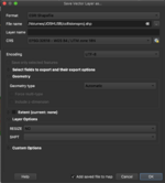
Now it's time to set the projection, to do so we will save those features with a new CRS:
- Go to where you have the layers, select that collisions vector layer and right click
- Hover over Export and then select "Save Features As"
- Choose a location to save it and name it so you can know what it is(e.g: collisionsproj)
- Select the WGS84/UTM Zone 18
- Options as shown on Figure 1 on the right
- Click OK
Projecting to a projection such as this one will be important considering we are dealing with distances when using the DBSCAN clustering.
Important: All vector data should be projected that way.
Symbology
We use symbology as a method of better reference. I would play around as you wish in the properties of the Wards, Collisions and Roads layer. To make sure there isn't too much colour similarities. I recommend to also do this post clustering as you will be classifying separate clusters with different colours. The next step will help us classify roads better.
Rule based classification
We decide to do a rule based classification to separate the highways from the main roads. To do that:
- Right click the roads shapefile and click on "Properties"
- Click on Symbology and in the drop down menu at the top select "Rule-Based"
- Under the only rule available, double click it, check the Filter box and click the purple dots next to the box(as shown in Figure 2)
- Enter ""SUBCLASS"='Highway'" in the Expression String Builder and then click OK(Settings should be like Figure 3)
- Then in the Label text box, label it "Highway"
- On that same page go down and select a symbol different to the roads you currently have.
- Click OK
- Click on the Green + at the bottom to add a new rule, double click, label it Roads and check Else as it's the other condition.
Applications
Once you are done setting up the environment, we can now start with the main purpose of the tutorial and that is the applications which will include classification and the usage of a concave hull. Once this is done we will have a good picture on how we can proceed in assigning areas to investigate collisions in Ottawa.
Clustering
Let's start with clustering, the tutorial, as already mentioned, will be going through two methods of clustering and how you can do those on QGIS. You need to be able to find those tools. Here is how you do:
- On QGIS, look for the processing toolbox on the right, if it isn't here go on the "Processing" menu on QGIS and select "Toolbox" and it should appear.
- You can now either search the search the tools of the aforementioned cluster methods which are "DBSCAN clustering" or "K-means clustering" or you can manually open the "Vector analysis" section of the toolbox and select them there(Shown in Figure 4)
Now that we have found the tools, I'll start explaining both methods starting with DBSCAN clustering.
DBSCAN clustering
Density based clustering in QGIS will help us find clusters based on the vector point densities in our collisions data set. This will use a minimum cluster size and a maximum distance between clustered points to give us multiple clusters and a good idea of what our areas could be. This would useful if you want to know how many officials you need based on some requirements that you would set.
Let's go step-by-step on how the tool works:
Note: As discussed earlier the tool only works if you've projected the data as done earlier
- Select "DBSCAN clustering" in the toolbox
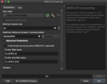
- You will get a window(as pictured in Figure 5) and you will select the projected collisions vector data you've created earlier
- You will then select a minimum cluster size and the maximum distance between clustered points as pictured(Stay in metres as it's the distance of units of the projected layer)
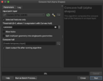
As mentioned earlier, DBSCAN clustering is incredibly particular with how it functions. It will take a lot of trial and error. On Figure 5, I have a combination of both that will yield you 15 clusters. All settings on that window should be as that figure shows to have that work
- Click OK
Figure 6 shows the results.
You will now have a new vector layer called "Clusters" with a table entry named "CLUSTER_ID". What is best to do next is to differentiate those clusters using colours and to do that:
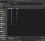
- Right click that new vector layer and select "Properties", a window like the one on Figure 7 will appear.
- Select "Symbology" and in the type of classification, select "Categorized"
- Underneath in the value box, select "CLUSTER_ID"
- Click on Classify below
- Click Apply
Each different cluster should have a differently coloured point symbol and then you just click OK and that is your DBSCAN clustering procedure done and you should ready to go to the next form of clustering.
K-means clustering
K-means clustering will create clusters based on the amount given so you tell QGIS how many you want and they will give you that amount. Useful if you already have a set of officials and you want to split them.
The steps are described below:
- Select "K-means clustering"
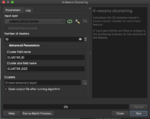
- You will get a window(as pictured in Figure 8) and select that same projected collisions vector layer from the other form of clustering
- You will then select a number of clusters that you want to separate the data in(as in the pictured example on that same Figure)
- Click OK
Figure 9 shows the results
To visualize the clustering, repeat the same steps to differentiate the colours as done in for the DBSCAN clustering. The result should be similar in terms of the coloured points we would get as a result despite the clusters being different in high likelihood.
Concave Hull
We have now got our clusters that we desire but we want the officials to get a region assigned. How can we get those regions traced out more clearly. We have create some vector layers which will be polygons that will contain the points in each cluster. You will do those steps for both DBSCAN and K-means methods as they will be identical.
To add those polygons we need to first select them by an expression:
- Right click on the Clusters
- Click on "Open Attribute Table"
- Click on "select features using an expression" which is in the icons over the attribute table
- Then you type "CLUSTER_ID"(it show start showing up once you start typing it) and "=0" which is the first cluster(as pictured on Figure 10)
- Click the "Select Features" button at the bottom of the window
Keep that window open and go back to your processing toolbox:
- Search "Concave hull" or go to Vector geometry and select "Concave hull(alpha shapes)"
You will see a window like on Figure 11
- Choose your Cluster that you worked on then check the "Selected Features Only" box
- Give the threshold 0.8 and uncheck the "Allow Holes" box.
- Click OK
You will then go back to the select by expression window and then change the CLUSTER_ID value to the next cluster and repeat for every cluster.
This should get you a polygon with a region for each official to go towards.
The outcome shown on Figure 12
Conclusion
The clustering methods in QGIS are very useful and relatively easy to use as shown in this tutorial. When using vector point data and there is a need for something to be divided, I think clustering does a good job at determining areas in which we can divide some tasks and for that it makes it an effective tool to use. I will say that the DBSCAN clustering method is incredibly particular and has given me some trouble to understand how it works. However, the solution to that issue which I have described is very straightforward and it is important to really follow the steps to use the tool. Doesn't matter if it's trying to investigate collisions or divide areas of garbageman using h ouse locations, that tool has incredible potential in terms of urban planning or any purposes where we would need to divide and conquer. It might not be as pronounced as the tool we have for ArcGIS but it is importantly a good open source alternative that will do the job when other more expensive software is not widely available.
Future Work
There definitely is a lot of future work in terms of the potential of something like this. You can add more components and maybe include some other GIS tools such as network analysis to calculate the most cost affective ways to investigate those areas(less gas consumption is better and could save city money). Use interpolation to maybe predict possible incidences of accidents. Future work more from a QGIS perspective is to include more methods of clustering as well. There is a lot that can be done around vector points that contain location data but that would be more suited for a separate tutorial not to overwhelm a user.
References
- Download Qgis. (n.d.). Retrieved December 20, 2021, from https://www.qgis.org/en/site/forusers/download.html
- Road centrelines. Open Ottawa. (n.d.). Retrieved December 20, 2021, from https://open.ottawa.ca/datasets/road-centrelines/explore
- Traffic collisions by location 2013. Open Ottawa. (n.d.). Retrieved December 20, 2021, from https://open.ottawa.ca/datasets/traffic-collisions-by-location-2013/explore
- Vector analysis. Vector analysis - QGIS Documentation documentation. (2020, June 5). Retrieved December 20, 2021, from https://docs.qgis.org/3.4/en/docs/user_manual/processing_algs/qgis/vectoranalysis.html
- Wards. Open Ottawa. (n.d.). Retrieved December 20, 2021, from https://open.ottawa.ca/datasets/wards/explore?location=45.249481%2C-75.800844%2C1.20
Very good support video k-means clustering:
- Kremer, Y. [Yannick Kremer]. (2017, February 4th 2019). QGIS Tutorial Unsupervised classification : K-means clustering [Video]. YouTube. https://www.youtube.com/watch?v=-wLCaRO44p4
