Exploring a subset of SAGA's Terrain Analysis tools
Purpose and Introduction
The purpose of this tutorial is to introduce the reader to a subset of the raster terrain analysis tools featured in SAGA GIS. Importing and Visualizing data will be discussed, and instruction will be provided regarding the functions of several of SAGA's Morphometry Terrain Analysis tools.
This tutorial will cover the use of basic digital elevation map analyis procedures such as finding the slope and aspect of a surface, more advanced operations such as analytical hillshading, plan curvature, vector terrain ruggedness, LS Factor and the automatic classification of landforms and landform elements.
Software
SAGA is a free and open source program which can be downloaded here: http://www.saga-gis.org/en/index.html
It runs on Windows or Linux operating systems, and can be run within a virtual machine.
Data
The data used in this tutorial are 1 m elevation data, though any digital elevation model (DEM) will work in this tutorial. Similar data can be found online on sites such as GeoGratis (http://geogratis.gc.ca/geogratis/en/search), and will be free and easily downloadable.
Tutorial
Importing data
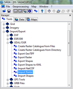
To import your data into SAGA you must enter the Tools section and select GDAL/OGR > Import Raster
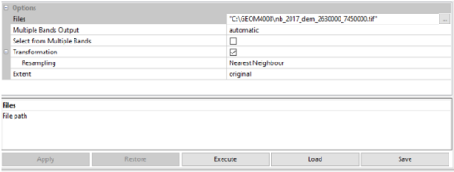
Select the 3 dots button beside files and select your file. Multiple Bands output is automatic but if you want to select specific bands check the Select from Multiple bands button below. Once everything is selected, hit apply and then execute.
Data visualization
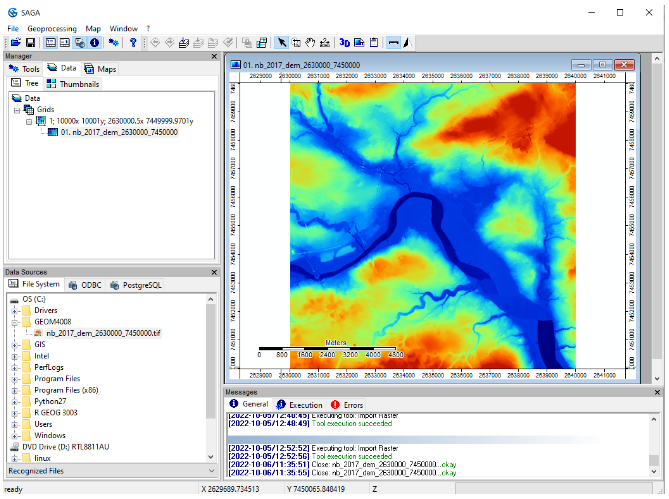
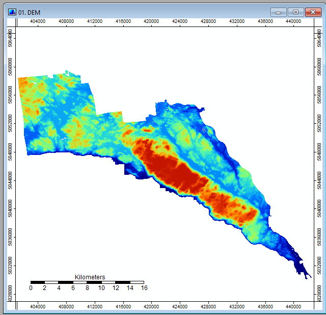
In the left window manager under data, right click on the data you have just imported and click "Add to Map", and the data will now appear in SAGA's view window.
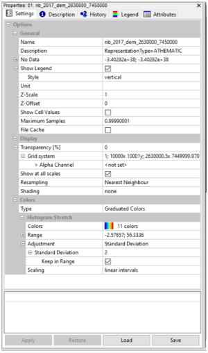
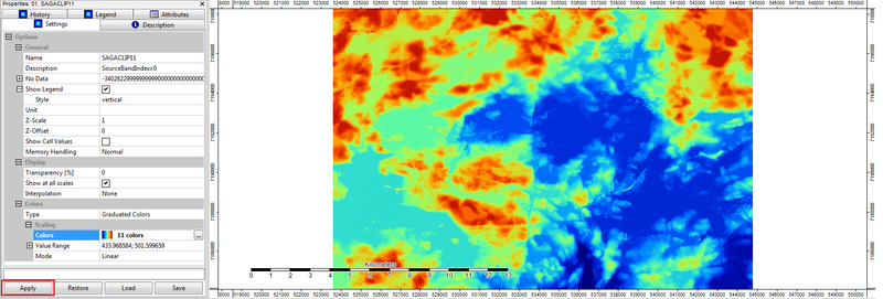
Depending on the raster uploaded it may come out with a colour scheme or in Greyscale. To better visualize the change in elevation, you can change the colour scheme by clicking the colour scaling option in properties. If the properties window pane isn't shown select this button: ![]()
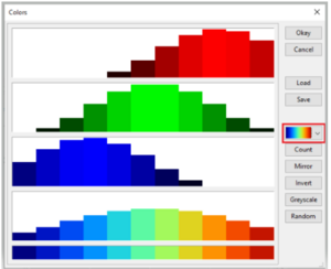
Next click on the colourful button to have more colour scaling options to choose from:
Finally select "Apply" and "Save"
Analytical Hillshading
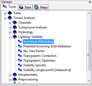
You will find the Analytical Hillshading tool under Terrain Analysis: Lighting, Visibility
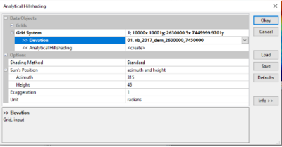
Within the tool window, specify the current grid system, as well as the elevation layer with the first imported data, and click okay:
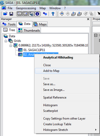
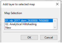
The output file will now appear in the Data tab under Tree. Right click the layer and select "Add to Map", making sure to add it to the initial map and not into a new window:
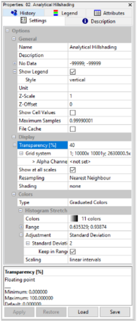
Next in settings change the transparency to 40% or however transparent you want the layer to be, so that both layers are visible and click Apply:
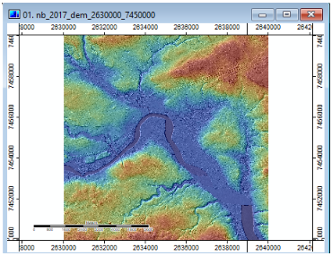
The resulting image should look like this:
Basic Terrain Analysis
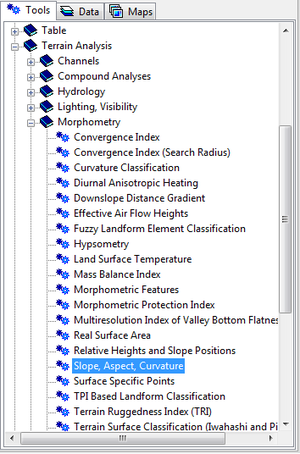
Within the toolbox, under Terrain Analysis: Morphometry, you will find the Slope, Aspect, Curvature function.
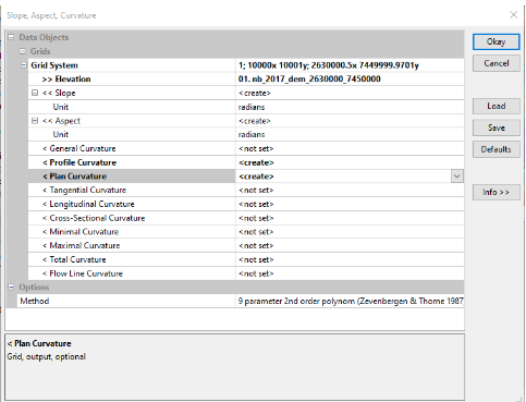
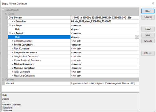
This is a batch process and it will produce 15 new fields at once. As seen below, enter the current grid system into the first field, the elevation data into the second field, check <create> for the fields Slope, Aspect, Profile Curvature, Plan Curvature and leave the remaining fields set to <notset>:
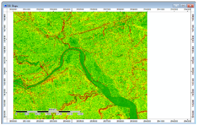
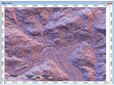
A subset of the results from this function are as follows:
Slope:
Aspect:
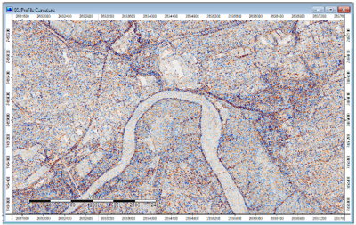
Profile Curvature:
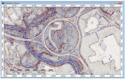
Zoomed in profile curvature:
Plan Curvature
The plan view curvature function found within the SAGA toolset is important for work in understanding variations in man-made and naturally occurring terrain. This tool can be used in fields such as road safety and maintenance, coastline monitoring, tracking mass wasting events, as well as watershed mapping.
Plan curvature by definition is the curvature in a horizontal plane. Positive curvature values indicate a convex contour within a cell, and negative curvature values indicate a concave contour within the cell, with respect to surrounding cells (http://www.et-st.com/et_surface/userguide/Raster/ETG_RasterCurvature.htm).
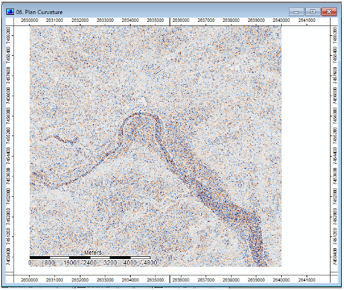
The resulting image for Plan Curvature is as follows:
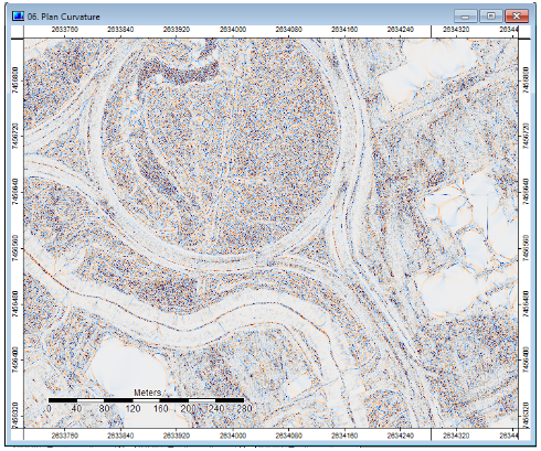
Zoomed in plan curvature:
In the plan curvature output blues represent a negative value (concave curvature), and red indicates a positive curvature (convex contour). The striated sections seen above in the output are over water and therefore have no definitive curvature, and are smooth in comparison. These areas could be removed to help the overall effectiveness of the map.
The small scale variation in curvature seen in the zoomed-in output above shows curvature variation in a low lying area. This information could be used to better understand the watershed and its extent.
Vector Terrain Ruggedness
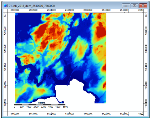
For the following instructions, a digital elevation file of St. John, New Brunswick was used.
Vector terrain ruggedness is a measure of the ruggedness of terrain, calculated by measuring the dispersion of slope vectors orthogonal to grid cells within a neighbourhood. In effect, this is a measurement of the combined variability in both slope and aspect. Ruggedness ranges between calculated values of 0, representing no terrain variation, to 1, representing complete terrain variation. Vector Terrain Ruggedness is primarily used in the study of animal habitat models [1]
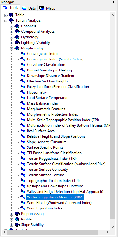
in SAGA GIS, Vector terrain ruggedness is calculated using the Vector Ruggedness Measure tool. It can be found under Terrain Analysis: Morphometry.
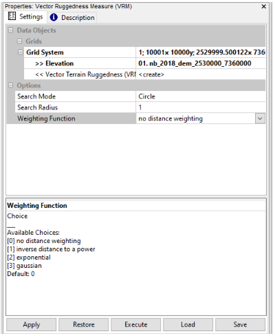
Within the tool window, specify the current grid system and the elevation map to be used for analysis. Set Vector Ruggedness Measure to <create> and make sure that Weighting Function is set to no distance weighting, after that press "apply", then "execute".
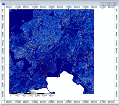
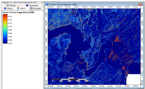
The resulting ruggedness measurement image is as follows.
As expected, the ruggedness is highest in areas with high variability in slope and aspect.
Fuzzy Landform Element Classification
For the following instructions, a digital elevation file of St. John, New Brunswick was used.
The Fuzzy Landform Element Classification tool uses fuzzy logic to approximate landform elements in an area. it is an unsupervised classification method that requires very little computing time compared to methods such as TPI Based Landform Classification. The analysis of landform elements is an important part of the field of geomorphometry [2]
To begin, use the Slope, Aspect Curvature tool to create slope, maximum curvature, minimum curvature, profile curvature and tangential curvature rasters from your DEM. Make sure the Slope Units field and the Aspect Units field are set to Degree.
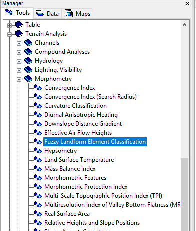
To begin the classification, select the Fuzzy Landform Element Classification tool from Terrain Analysis: Morphometry
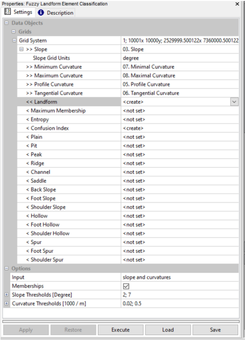
Then, enter the rasters that you created in the previous steps into their appropriate fields, making sure Landforms is set to <create>, memberships is selected at the bottom, then hit "apply" then "execute".
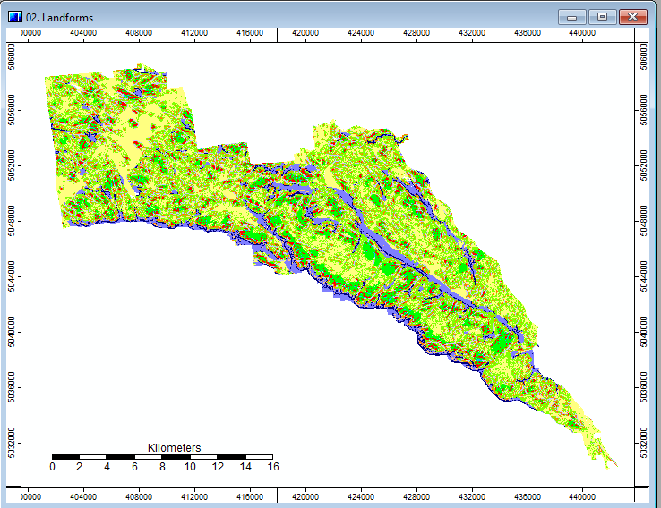
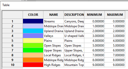
The raster labeled "Landform" contains the now-classified landform elements. The classified landform raster should look like this with a legend with labels is found in the side panel.
TPI Based Landform Classification
For the following instructions, a digital elevation file of Gatineau Park was used.
Topopgraphic position index, or TPI,is an algorithm for determining an object or point's relative topographic position to a landform. TPI works by comparing the value of each cell in a DEM with the mean value of its neighbourhood. Positive values indicate areas of relatively high elevation, like ridges. Negative values indicate areas of relative lows, like valleys. Values close to zero indicate areas of constant slope. TPI depends heavily on the scale of the analysis, with smaller scales providing significantly less detail. combining both small and large scale TPI allows for the classification and interpretation of many landforms. is useful in that many processes acting upon natural landscapes are heavily influenced by relative topography, and API provides a means of measuring topographic setting [3].
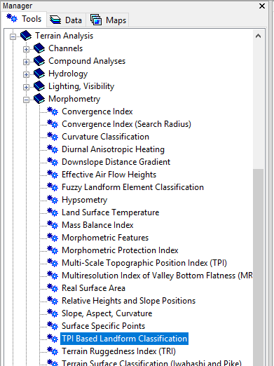
In SAGA GIS, the TPI interpretation of landforms is accomplished with the TPI Based Landform Classification Tool, found under Terrain Analysis:Morphometry.
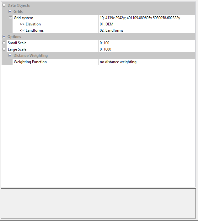
The TPI Based Landform Classification Tool only requires a DEM to function. Depending on available processing power and the resolution of your DEM, geoprocessing can take a long time. Enter the DEM into the Grid System and Elevation fields in the appropriate fields, as shown below:
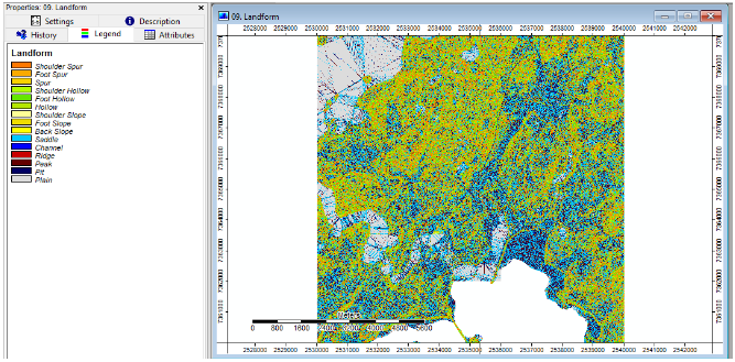
Once geoprocessing is complete, the output should resemble the image below
A labeled classification scheme for the created raster is automatically generated. It can be seen below
LS Factor
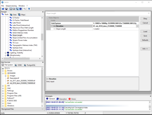
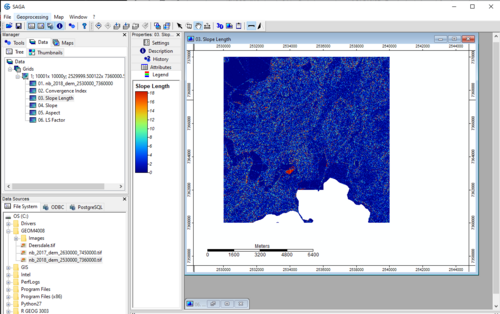
The LS factor uses Slope Length and Slope to help predict erosion potential. LS Factor is useful for soil erosion, soil loss and other losses caused by erosion (HRABALÍKOVÁ1, 2017). To use this tool first we have to create the Slope Length. Go into Tools > Terrain Analysis > Hydrology > Slope Length. Add the current grid and the DEM as elevation. This tool takes some time to process so be patient.
The results should look like this:
To create Slope: found in Terrain Analysis > Morphometry > Slope, Aspect, Curvature. Select <create> for slope. As done above in Basic Terrain Analysis section.
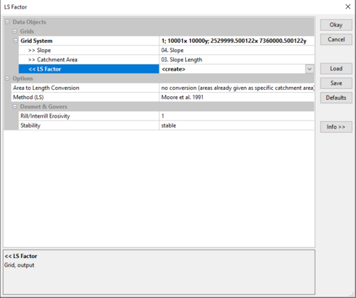
Once slope is created go to LS Factor which is found in Terrain Analysis > Hydrology > LS Factor. Plug in the grid system you are using and your create slope for slope and slope length under Catchment Area.
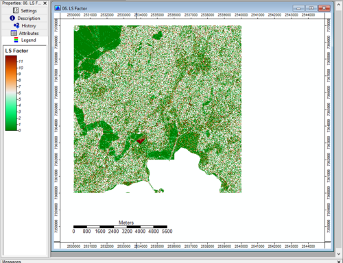
The LS results will look like this and you can look at the legend in the window pane to the left of the map.
Reference
Hengl, T., & Reuter, H. I. (2013). Geomorphometry: concepts, software, applications. Retrieved from https://books.google.ca/books?id=u33ArNw4BacC&lpg=PA227&ots=h9MkkvRK_B&dq=geomorphometry%20landform%20elements&pg=PA227#v=onepage&q&f=false
SAGA software: http://www.saga-gis.org/en/index.html
Service New Brunswick, (2017). Retrieved from: https://geonb.snb.ca/nbdem/index.html
Service New Brunswick, (2018). Retrieved from: https://geonb.snb.ca/nbdem/index.html
Sappington, J.M., K.M. Longshore, and D.B. Thomson. 2007. Quantifiying Landscape Ruggedness for Animal Habitat Anaysis: A case Study Using Bighorn Sheep in the Mojave Desert. Journal of Wildlife Management. 71(5): 1419 -1429 [4]
GeoGratis: http://geogratis.gc.ca/geogratis/en/search
http://www.et-st.com/et_surface/userguide/Raster/ETG_RasterCurvature.htm
Weiss, A.D. (2000): Topographic Position and Landforms Analysis. poster. [5]
HRABALÍKOVÁ1, M. and JANEČEK1, M., (2017). Comparison of Different Approaches to LS Factor Calculations Based on a Measured Soil Loss under Simulated Rainfall. Retrieved from: https://www.agriculturejournals.cz/publicFiles/222_2015-SWR.pdf
Social Saga, (2022) Saga GIS Tutorials. Retrieved from: https://sagatutorials.wordpress.com/basic-terrain-analysis/
