Exploring terrain analysis using Quantum and GRASS GIS
Contents
Purpose
The following tutorial was developed as a course requirement for GEOM 4008 - Advanced Topics in GIS at Carleton University. It informs the user on basic preliminary data manipulation of terrain and topological data. This tutorial should serve to explore and visualise your data prior to more rigorous analysis.
Introduction
As the field of Geomatics continues to grow, so does the multitude of Free and Open Source Software for Geospatial tools (FOSS4G). While the functionality of such tools may not be as advanced as some proprietary software, they carry two distinct advantages:
- Free - software may be used, studied, modified and distributed without restriction
- Open Source - the source code is available to the general public for use and/or modification
When combined with freely available spatial data, FOSS4G tools may perform a variety of powerful functions including geospatial analysis, Digital Elevation Models (DEM), network analysis, etc.
The following tutorial was developed to demonstrate the use of FOSS4G tools and free data to perform a variety of standard terrain analyses. Using Quantum (version 3.8.3 "Zanzibar") and GRASS (version 7.4.1) GIS software this tutorial will show how to:
- Download free DEM tiles and other reference data layers from Open Data, the government of Canada open data portal
- Identify and import different topographical data formats
- Merge multiple tiles to form a continuous DEM
- Clip reference layers to match the study area
- Create Slope, Aspect, and Hillshade maps
- Generate custom Contour maps
- Ruggedness Index (Quantum)

Methods
Quantum GIS
Getting Started: Acquiring Software and Data
Step 1 - Downloading Quantum and GRASS GIS
To begin, ensure you have both QGIS and GRASS installed on your computer. They can be downloaded as part of the OSGeo software package OSGEO-Live, and are available for a variety of operating systems such as Windows, Linux, and MacOS X. Click here to go directly to the Quantum GIS download page.
Note - all menus, tool names, or other references were gathered while running the software on a Microsoft Windows platform.
Step 2 - Finding Free Data
All data in this tutorial were retrieved from Open Data, an initiative "implemented to increase the availability of base geospatial data to all Canadians".1 Open Data is a reliable source for a variety of high-quality Canadian data including:- Administrative Boundaries
- Digital Elevation Data
- Land Cover
- National Road Network
- Satellite Imagery
This example uses 1:50,000 scale DEM data near Thunder Bay, Ontario. Click this link to access the Open Data data selection tool. Choose NTS areas 052A06 and 052A11, then Submit. Click the http link next to each dataset to download it. Save everything into a project folder (i.e. Terrain_Analysis_Tutorial).
While it is not strictly necessary, having reference data is always useful to help provide cartographic context. In this case, download the National Road Network data for Ontario in ESRI Shapefile format (under the "changes between editions" heading) here. This may take a few minutes to download. Take a second to look through the files. Notice that there are layers for things like "Toll Points" and "Ferry Segments". Feel free to delete these files as they are not required. Keep only the files with "ROADSEG_MODIFIED" in the name, plus the Readme. This will be easier to work with.
NOTE - You will have to create a username, have a valid e-mail, and login to download data. Don't worry, anyone can do it. Also know that some data sets may be e-mailed to you and not directly downloaded from the Open Data portal.Data formats
Rarely will your data come directly packaged in a .dem format. You will often be working with .tif files for elevation data or even vector data that you will need to convert to a raster format. This section will go through the most common data formats and how to import them into QGIS and where the different conversion tools are located so that you can manipulate your data using the tools outlined in this tutorial. Before doing any sort of data analysis you should evaluate the quality of your data. Some data come with large areas with no data. Others are derived from spot elevation models that give an incomplete view or interpolate the true topography of a region and are not based on direct measurement. Whatever the case, look at what ever metadata is available and identify the limits of your data.
Raster data (.tif, .dem, etc.)
Importing raster data is straight forward, Layer » Add Layer » Add Raster Layer.... However note that importing .dem and .dsm data directly does not work with base QGIS. you will need to import your raster data in .tif or another raster format.There are also a number of conversion tools to convert raster to vector, Raster » Conversion » Polygonize... and vector to raster, Raster » Conversion » Rasterize....
Consider the tools to convert your raster data to a different raster format, Raster » Conversion » Translate.
Also always make sure your projections match for every data layer and make sure it is an appropriate projection, Raster » Projections » >>> .
Vector data (.shp, kml, kmz, etc.)
Topological vector data usually come in the form of contour poly line or spot height elevation data. If you plan on using vector data to do the terrain analysis in this tutorial you will need to convert it to a raster tiff data format. To import your vector data, Layer » Add Layer » Add Vector Layer...
Delimited text (.txt, excel, etc.)
When importing these data sets, Layer » Add Layer » Add delimited text layer..., you can import them directly as a table or as a vector layer. If you decide to import it as a vector layer you will need to make sure your X and Y coordinates correspond to latitude(Y) and longitude(X).
Web sources (wms, databases, ect.)
Web sources allow you to directly import large data sets from private and publicly available data, Layer » Add Layer » Add WMS/WMTS layer.... There are numerous kinds of web services that allow you to do this. Consider that some of these data sets may not be read only and not allow for many analysis options.
CAD data (.dwg)
In some cases topological data will be given to you in a .dwg format. This is the format used by CAD and in these instances the topological data is paired with extensive data on surrounding feature. Typically there will be base topological features (contour lines) and numerous surface and subterranean features such as trees, building, pipes, ect. Ususally in a vector format. To import these files go to Project » Import/Export » AImport Layers from DWG/DXF.... This will import all layers associated with the file. Only use the relevant contour layer.Viewing DEM tiles
Start by opening QGIS and loading the DEM tiles. Despite downloading DEM's for only 2 areas, there are 4 tiles to add (see below).
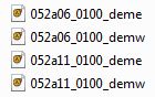
Note that each area is sub-divided into 2 tiles; East and West.
Together, these 4 tiles will form a square study-area.
Once you have added all 4 tiles, the map should look like Figure 1 (yes, a grey square). Don't worry, this is correct. To get it looking like Figure 2, apply a contrast enhancement to the display properties for each tile.
- Double-click a layer in the table of contents to open the Properties window
- Under the Contrast Enhancement section, choose "Stretch To MinMax" from the drop-down menu
- Repeat for all 4 tiles

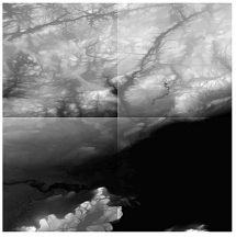
Figure 1: DEM tiles when
first loaded in to QGISFigure 2: DEM tiles with
contrast enhancement
It is also helpful to see the DEM in colour. Using the same process as above, open the Properties window. This time, change the Colour Map to Pseudocolour. The map should now look like the one below.
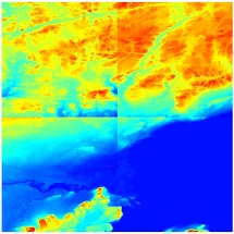
Figure 3: DEM tiles with
pseudocolour display
Merging DEM tiles
Performing a merge on the 4 DEM tiles will accomplish two things:
- Output map will appear nicer - no lines running through the middle
- Terrain analysis can be performed on one continuous DEM as opposed to four separate ones
Quantum has a tool designed specifically for this task. Find the "Merge" tool under the Raster » Miscellaneous menu.
Use the following parameters:- Input Files: Navigate to the folder where you stored the DEM files and select all four
- Output File: Specify a file name and location for the merged DEM (i.e.DEM_Merge)
- Load into canvas when finished: Check this to load output map into table of contents
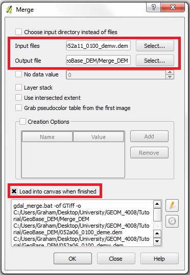
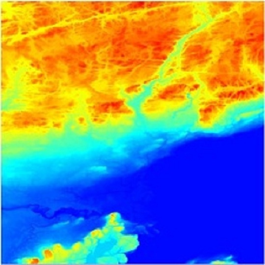
Figure 4: Merge tool parameters Figure 5: Merged DEM map
Adding and manipulating reference data
Now that the DEM looks nice, it may be useful to add some reference data. Click the "Add Vector Layer" button.
 Navigate to where you saved the Ontario Roads shapefile (.shp) earlier and add it.
Note - It may take a minute or two to show up. This is because the file contains road segments for ALL of Ontario, and is therefore quite large. Once it shows up, right-click on the roads layer in the table of contents and choose "Zoom to Layer Extent" (Figure 7).
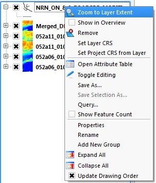
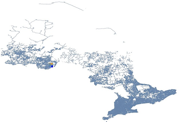
Figure 6 Figure 7: Extent of Ontario road segments shapefile
Clearly, we do not the road segments that are outside of the DEM; they only serve to slow things down. This can be accomplished using the Clip tool. Unfortunately, we cannot clip a vector layer (roads) using a raster layer (the DEM). We will have to create a new vector layer to match the extent of the DEM.- Click the "New Shapefile Layer" button

- Choose a Polygon type, and click OK
- Specify a file name and save it in the same folder as the other data. I chose AOI.shp (Area Of Interest)
The new layer will now appear in the table of contents. Right-click and select "Toggle Editing". This allows new features to be created for the layer. Next, find the "Add Feature tool" on the Digitizing toolbar.
Note - if the toolbar is not visible, toggle it on under the View » Toolbars menu).
Draw a square polygon by clicking on each corner of the DEM. Right-click to finish the polygon and give it an ID of 1. Don't worry about being precise - you can always use the "Node Tool" to edit the vertices. Save the edits
  and toggle editing off.
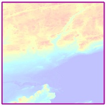
Figure 8: New AOI layer
(purple square)
Now, clip the Ontario roads layer to the newly created AOI. This will create a new layer (a subset of the roads layer) that only includes features situated within the AOI.
The Clip tool may be found under the Vector » Geoprocessing Tools menu. Use the following parameters:Table 1: Clip tool parameters Parameter Description Input vector layer - Roads layer to be clipped [NRN_ON_8_0_ROADSEG_MODIFIED]
Clip layer - The extent to which we went to clip the roads [AOI_Polygon]
Output shapefile - Pick a meaningful name for the new layer [Roads_clipped.shp]
The map should now look something like Figure 9.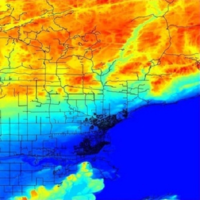
Figure 9: DEM with clipped roads layer
Slope and Aspect
Slope maps characterize the degree of terrain slope (typically in degrees) and are excellent for a "quick interpretation of land systems."2
Aspect maps display the cardinal direction of a slope face (i.e. North, West, etc.).3Both the Slope and Aspect tools may be found under the Raster » Terrain Analysis menu (ensure the Terrain Analysis plugin is enabled). Use the following parameters:
Table 2: Slope and Aspect map creation parameters Parameter Description Elevation Layer - Select the merged DEM
Output Layer and
Output Format- Define a new file name
- Save it as a GeoTIFF
Z factor - Use the default value of 1.0
Add result
to project- Check this to add the new layer
directly into the table of contents
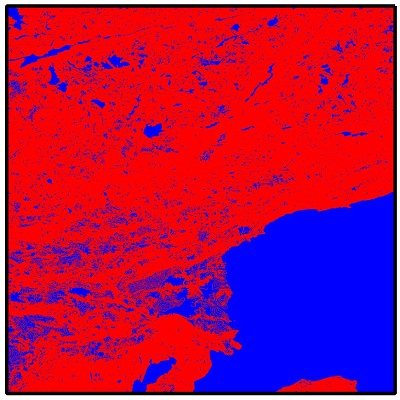
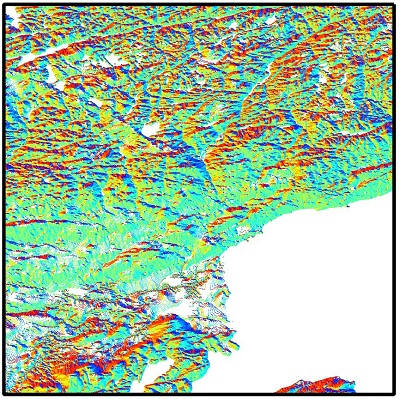
Figure 10: Slope Map Figure 11: Aspect Map.
Colours represent the direction of slope face.
Note - clearly, the slope map is incorrect. At the moment it appears to be a binary representation of areas with a slope of zero (blue) and areas with a slope greater than zero (red).
I think this is just an issue with symbolization. I have, however, explored many different options and haven't yet found one that is appropriate. Any feedback on this matter is appreciated.Hillshade
Hillshade maps are typically created for cartographic effect and can make a 2D map appear 3D. Lighting effects are added based on variations in elevation. This is intended to mimic the effects of the sun shining on a landscape (illumination, shadows, etc.) 4
The Hillshade tool can be found under the Raster » Terrain Analysis menu.
Table 3: Hillshade map creation parameters Parameter Description Elevation layer - Select the merged DEM
Output layer
& format- Define a new file name
- Save it as a GeoTIFF
Z factor - Use the default value of 1.0
Add result to project - Check this to add the new layer
directly into the table of contents
Azimuth - Use the default value 300
Vertical angle - Use the default value of 40
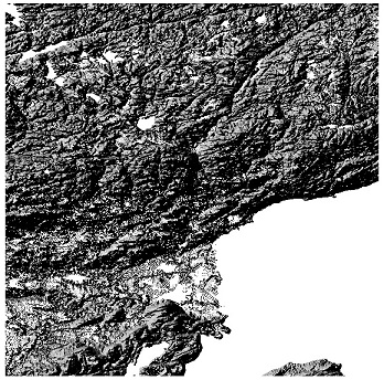
Figure 12: Hillshade map Contour Maps
A contour is a line that connects "a series of points of equal elevation and are used to illustrate topography, or relief."5
Elevation is represented at defined intervals above sea level (typically feet or meters). The distribution of contour lines allows for a quick interpretation of the landscape:- Where contours are close together, the slope is steep
- When contours are far apart, the slope is more gradual
In Quantum GIS, find the contour tool under the Raster » Extraction menu.
Table 4: Contour map creation parameters Parameter Description Input file (raster) - Select the merged DEM
Output file - Define a new file name
Interval - Try several different intervals
Load into canvas
when finished- Check this to add the new layer
directly into the table of contents
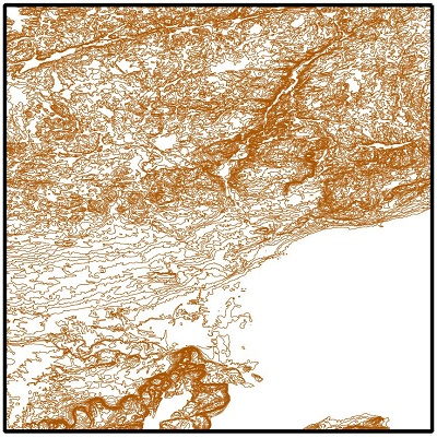
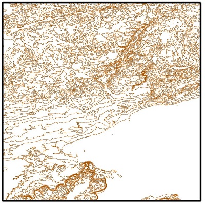
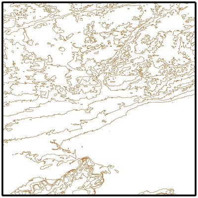
Figure 13a: 10m Quantum contour map Figure 13b: 20m Quantum contour map Figure 13c: 50m Quantum contour map
Ruggedness Index
This is a unique tool that calculates terrain heterogeneity based on the change in elevation between a grid cell and its neighbouring cells.
"Terrain heterogeneity is an important variable for predicting which habitats are used by species and the density at which species occur across a variety of environments." 6
The Ruggedness Index tool may be found under the Raster » Terrain Analysis menu.
Table 5: Ruggedness Index parameters Parameter Description Elevation Layer - Select the merged DEM
Output Layer/Format - Define a new file name
- Save it as a GeoTIFF
Z factor - Use the default value of 1.0
Add result to project - Check this to add the new layer
directly into the table of contents
In the development of this index, results were interpreted as follows:Table 6: Interpretation of ruggedness values Sum Change
in Elevation (m)Description 0-80 - Level
81-116 - Nearly Level
117-161 - Slightly Rugged
162-239 - Intermediately Rugged
240-497 - Moderately Rugged
498-958 - Highly Rugged
959+ - Extremely Rugged
Note - The values above may be misleading because they were applied to a specific case study. For the ruggedness map below, areas become increasingly rugged as they change from light blue to yellow and to red.
Notice the clear outline of the mountain overlooking Thunder Bay at the bottom left of the map.
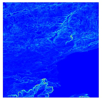
Figure 14: Ruggedness Index
GRASS GIS
Getting Started: Acquiring Data
At this point you should already have GRASS installed on your computer. If not, please refer to section 3.1.1 (Getting Started: Acquiring Software and Data).
Data acquisition for this portion of the tutorial is not the same as for previous sections - we do not need to find and download the raw data again. We have already done the work to merge 4 DEM tiles into 1 continuous DEM, and to format the reference data. All we need to do is import these files into the GRASS file format.
First, create a new folder in your file directory to store GRASS data files (i.e. GRASS DATA).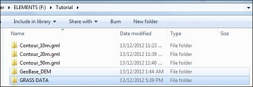
Open GRASS. In the "Welcome" screen you are asked to define the following:Table 7: GRASS GIS project parameters Parameter Description Action GIS Data Directory Tells the program where to find your data - Navigate to your newly created "GRASS DATA" folder
Project Location A project - defined by its coordinate system,
map projection and geographical boundaries- Click the Location Wizard button and define a new location called Thunder Bay
- Choose the "Read projection from a georeferenced data file" option
- Navigate to and select the Merged_DEM file we created earlier in Quantum
Mapset A sub-project. Each location can have many mapsets - Click the Create Mapset button and name it Tutorial
Click Start Grass . Notice that the GUI (Graphic User Interface) is a little bit different than Quantum. GRASS uses multiple windows to display information. Three basic windows will appear on start-up:- Command prompt: all tasks can be performed here, but it is often nice to use a GUI
- Layer manager: contains table of contents (called map layers) and all tools for adding, editing or otherwise manipulating data
- Map display: displays active data layers and provides viewing options (zoom level, adding map elements, etc.)
First, we need to import the Merged_DEM file we created in Quantum. In the Layer Manager window under the File menu, choose Import Raster Data » Common import formats- Click the Browse button and navigate to the Merged_DEM file. Make sure to select "All Files" in the drop-down menu (Figure _)
- Import the file. GRASS will automatically save the file in its own format in the GRASS DATA folder
- To view the new layer, toggle it on in the Layer Manager
- Repeat the process to import the reference data (Import vector data, see Figure _)
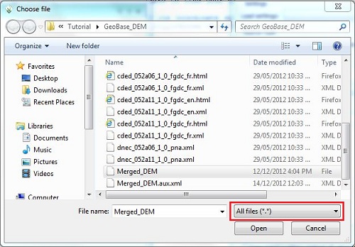
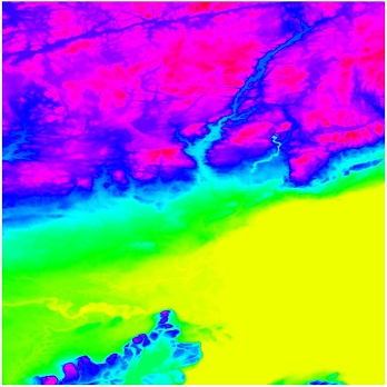
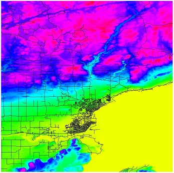
Figure 15: Adding a raster file to GRASS Figure 16a: GRASS display of Merged_DEM Figure 16b: Merged_DEM with reference data
Note - You may want to change the colours so that it more closely resembles the DEM as displayed in Quantum.- Right-click the layer in the table of contents and select Set Colour Table. In the Colours tab, select byr from the drop-down menu (blue-yellow-red)
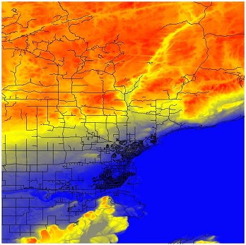
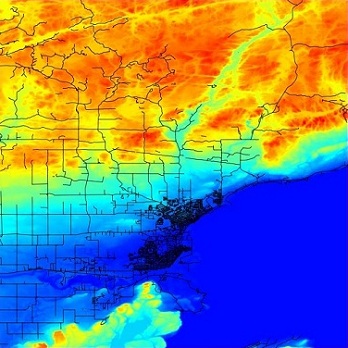
Figure 17a: Recoloured GRASS DEM Figure 17b: Quantum DEM
Slope and Aspect
Both of these maps can be created in the same step using the Slope and aspect (r.slope.aspect) tool under the Raster » Terrain Analysis menu.
Table 8: Slope and Aspect map parameters Parameter Tab Description Required - Select Merged_DEM
Outputs - Define a name for the output slope and aspect maps
Settings - Use defaults (no change)
Optional - Use defaults (no change)
Note - the aspect map will initially appear in greyscale. Change the colour table (as described above) to aspectcolr.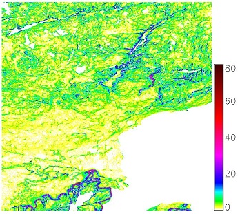
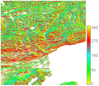
Figure 18: GRASS Slope Map Figure 19: GRASS Aspect Map
Hillshade
The GRASS hillshade tool is called "Shaded Relief" (r.shaded.relief) and can be found under the Raster » Terrain Analysis menu.
- Use the same vertical and horizontal angle parameters as we did in Quantum (the defaults) so we can compare the output maps
Table 9: Shaded relief map parameters Parameter Tab Description Required - Select Merged_DEM
Optional - Define a name for the output map
- Altitude of the sun (vertical angle): 40
- Azimuth (horizontal angle): 300
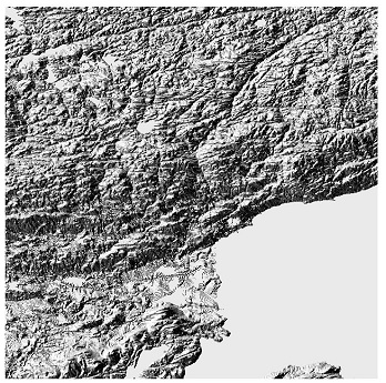
Figure 20: GRASS Shaded Relief Map
Contour Maps
The GRASS contour tool is called "Generate contour lines" (r.contour) and can be found under the Raster » Terrain Analysis menu.
Table 10: Contour map parameters Parameter Tab Description Required - Select Merged_DEM
- Define a name for the output map
Optional - Define the contour interval (increment)
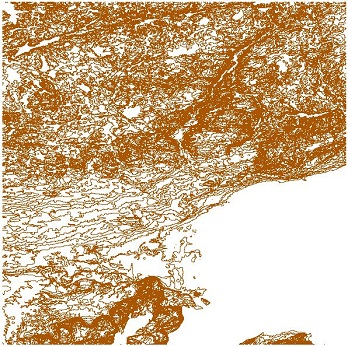
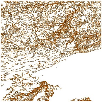
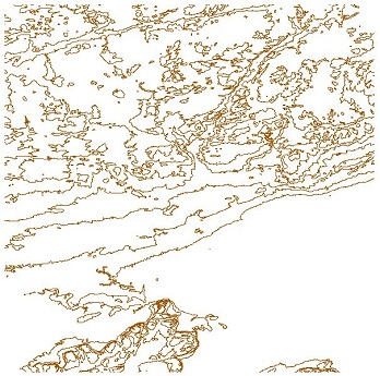
Figure 21a: 10m GRASS contour map Figure 21b: 20m GRASS contour map Figure 21c: 50m GRASS contour map
Discussion & Conclusion
Through this tutorial you have explored the use of FOSS4G tools and free data sources to perform basic terrain analysis. Using both Quantum (version 1.8.0 "Lisboa") and GRASS (version 1.6.4) GIS software you have created:
- Slope and Aspect maps
- Hillshade/Shade Relief maps
- Custom contour maps at varying intervals
Quantum and GRASS are different in many ways.
- GUI (Graphic User Interface)
GRASS uses a windowed GUI while Quantum displays everything in a single window with menus and toolbars - File Structure
GRASS automatically saves files in its own native format, all in a single data folder. Quantum can draw data files from any number of locations. - Geoprocessing and other tools
GRASS comes loaded with more tools than Quantum. Both rely heavily on the use of plugins for additional tools
While there are numerous differences it has been shown, using this tutorial as a guide, a user may perform the same basic terrain analyses in either program.References
1 - Open Data (2019). Open Government. Government of Canada
2 - Denness, B., Grainger, P. (1976). The preparation of slope maps by the moving interval method. Area, 8(3), 213-218.
3 - Intermap (2012). Slope and aspect maps
4 - Land Trust GIS (2011). Making effective use of shaded relief
5 - Natural Resources Canada (2007). What are contours?
6 - Riley, S., DeGloria, S., Elliot, R. (1999). A terrain ruggedness index that quantifies topographic heterogeneity.Intermountain Journal of Sciences, 5 (1-4), 23-27.


