Interpolating a surface and determining overland flow distance via qGIS and SAGA GIS

Purpose

The purpose of this wiki is to introduce users to the cross functionality of open source software. It is intended to show how a user can take raw elevation data and create a usable GIS product within a short time period, as to realize geographic phenomena in real world situations such as a spill mitigation scenario.

Introduction

The direction of this project is to show how free and open source software for geospatial applications (FOSS4G) can be implemented as an alternative and in some cases an enhancement to licensed products such as IDRISI and ESRI's ArcMap. To portray this both QGIS and SAGA GIS will be used. The purpose for using two programs is due to ease of use. Where QGIS allows for easy operations to be performed in a somewhat familiar GUI, it does not account for more in depth applications such as flow direction of liquids and the distance they must travel before entering a major tributary. Thus, this tutorial aims to show how to take vector elevation data and transform it to a raster surface which is conducive to modelling and extrapolation.

Software Download and Data Gathering

To download the necessary programs for the purpose of this tutorial, click the following link for the QGIS download portal[1]. It is recommended that you download QGIS Standalone Installer version 3.16 (as this is the most stable version of the software). However, you may download the latest version of the software if you feel comfortable doing so. The link for SAGA GIS's download portal can be found at [2]. You will see a link on the left hand side of the page under @SourceForge called downloads, click on that. This will take you to the download link, simply download and install the a version of the software (Version 8.0 is the newest, however Version 7.0 is more stable). Upon downloading and installing the correct version as it corresponds to your computer, the next step is to find suitable data for analyzing the area of study. Among many sources, elevation data for Canadian areas can be found easily through such outlets as the government of Canada website, under open Canada at the following link [3]. This site will allow you to search through a wide range of ferally open data sources and catalogues. Alternatively, you could use a site that is more specific to your area of interest. Such as Data Ontario, which will allow you to search through a variety of data sources and catalogues for Ontario. Of course all other Provinces have their own version of this site. Data Ontario can be found at this link [4].

Methods

The project can be divided into two steps: performing the surface interpolation in QGIS and using that produced DEM to determine the overland flow distance in SAGA GIS.

Surface Interpolation in QGIS

The first step is to get QGIS running. Click on the Q emblem placed on your desktop, and upon loading press skip to close the tips menu. Having acquired the data, the elevation points should be brought into QGIS via the add delimited text layer tool found under the “layer” tab on the taskbar.

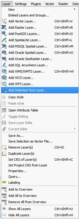
Once you are in the add delimited text layer, simply name the layer as you see fit and toggle on the specifications of the input data table so that it displays properly at the bottom of the screen, as in the following picture:

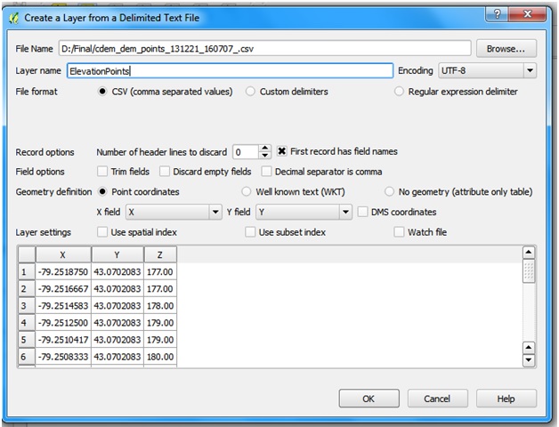
You will now have a block of points the size of your study area. In order to make these points into an interpolated surface we must use the "interpolation" tool under the raster tab, as follows

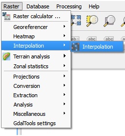
Once in the interpolation window, we find a series of options. Set the interpolation value to that of the elevation value of your dataset, in this case it is column z. If you aren't sure which column is the elevation values, look up the table in excel or open the meta data which came with your elevation points to determine which column it is. For the purposes of hydrology, an IDW interpolation is best so we select it as such. Cell size is perhaps the most important attribute to select: set it too big and the resultant map will be complex and take quite a while to process, set it too small and you will see generalization and a lack of interpretation abilities. You should try starting small and moving towards big to determine the optimal size. The window should look something like the following:

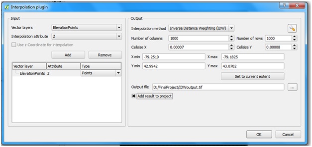
Determine where you would like to save the image and click okay when you are satisfied with the parameters you have selected and you will see this window:

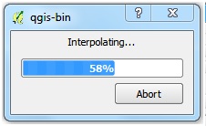
Once processing has finished, dependent on the size of your data set this could take a few minutes or multiple hours, you will see an interpolated surface automatically appear on your map, such as the following:

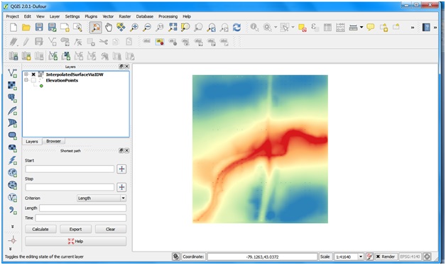
Voila! We have created an interpolated surface. Now we move to SAGA GIS to perform a more in depth analysis.

Alternative Method of Interpolation in QGIS

Another method you could use to add the desired layers into QGIS would be to: simply navigate through the Browser to the files you wish to add on the left hand side of your screen. Find the correct file directory to where you have saved these files, then simply drag them onto your map. (note: I will be using a different data set to run this interpolation, but follow along with whatever data you have, as long as you have some elevation data!)

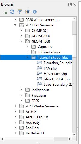
Now, you should be able to see your data displayed on the map, as well as see the layers displayed in the layers tab.

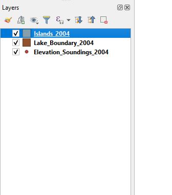
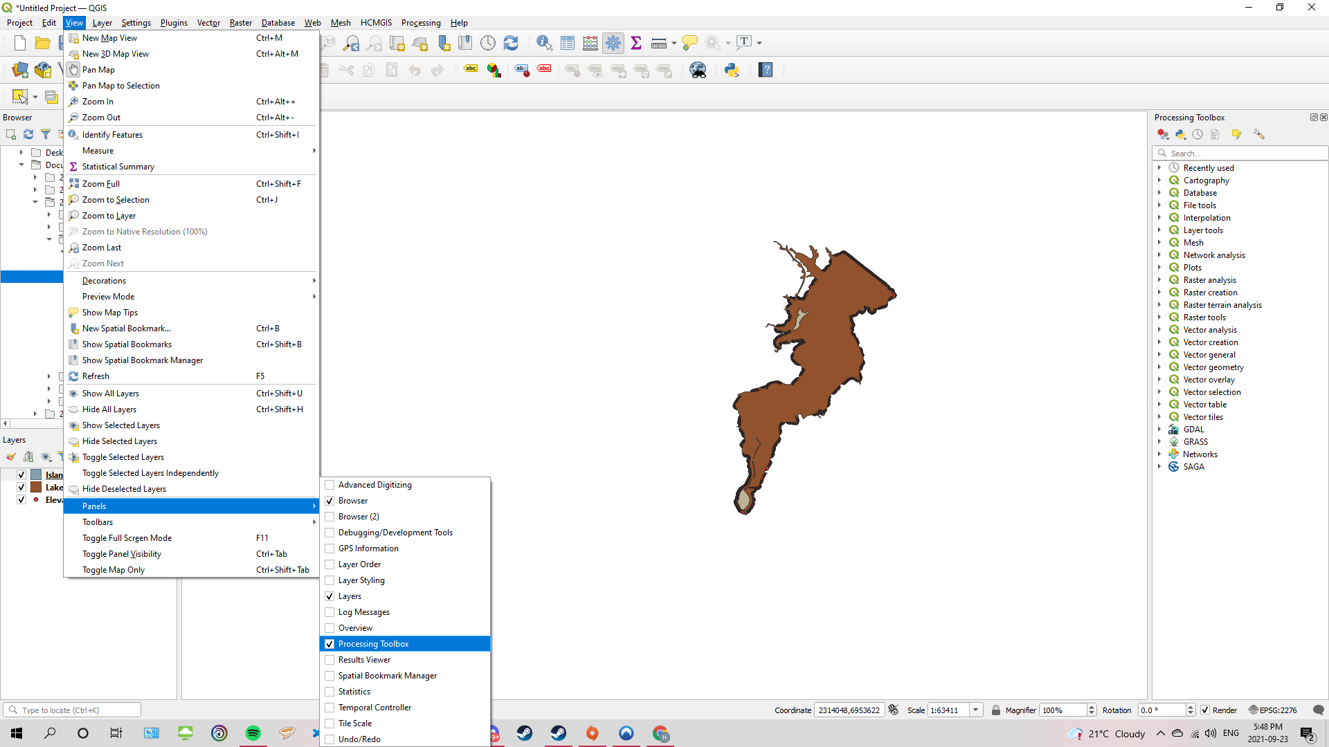
With this step done you can now begin the process of interpolation. Scroll over the the tools bar in the right hand corner of your screen. If this has not already been opened then simply open the panels section under the view tab at the top of your screen. Once there select the processing toolbox. This will activate and lock the toolbar to the right of your screen.

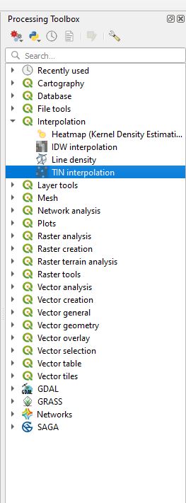
Now, simply click on the "interpolation" option in the toolbar. This will display 4 different options. The ones that we are interested in this tutorial are "IDW interpolation" (Inverse Distance Weighting) and "TIN interpolation" (Triangulated Irregular Network). Both are great in their own aspects, TIN interpolation is more typically used for elevation data. Whereas, IDW interpolation is used for more general things, such as populations or landcover or temperature and etc. In this case since we are using evaluation data, so we will be creating a TIN interpolation. So, simply click on the TIN interpolation symbol.

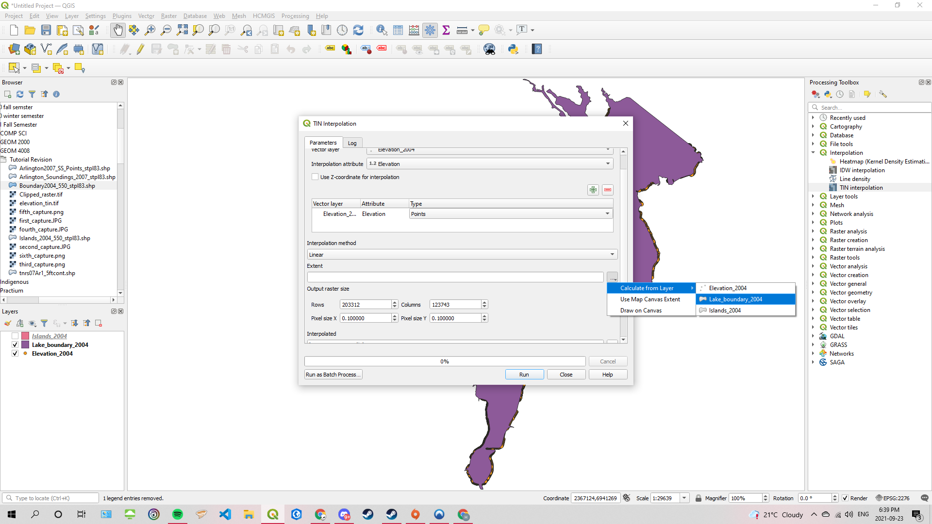
With this new textbox open, select the layer you wish to interpolate on the vector layer tab. Then be sure to change the interpolation attribute to the category in your selected layer that contains the elevation data. Next, click the green plus symbol and make sure the TYPE is as points. You will need to add an extent. To do so click on the three dots beside the extent tab, in this case I will set it as the boundary shapefile I have for the lake I am using.

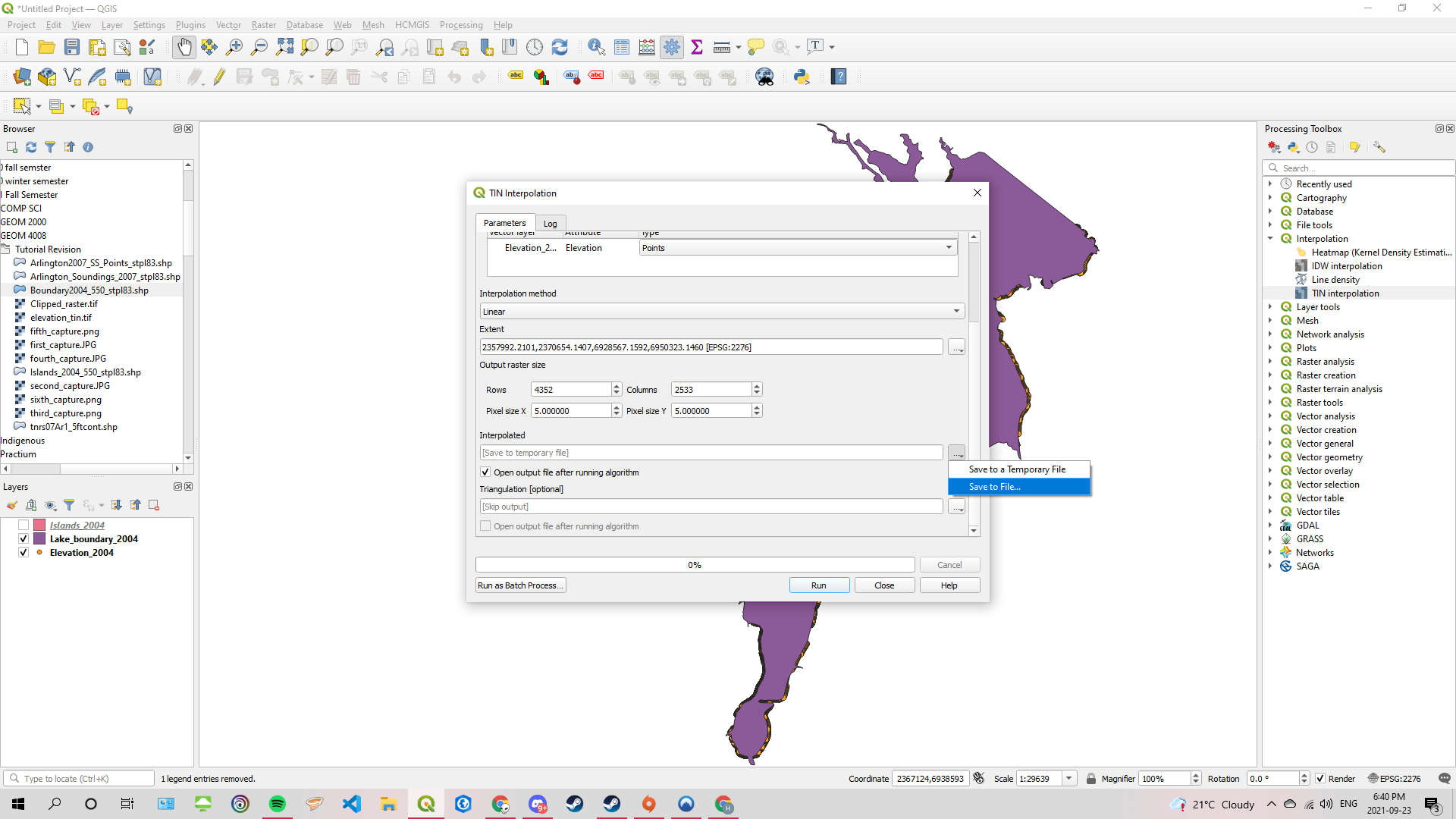
Next, you will want to set the pixel size for this interpolation (this is the same thing as cell size, just different term for it). As said above, if you set this too large then the map will become complex and take LITERAL hours to load, too small and it will be too generalized. Play around with these numbers to find one that works for you, In my case I will be setting them to 5. Lastly if you want to make this a permanent shapefile then click the three dots beside the interpolated tab at the bottom of the textbox. Click "save to file" and name the file, but MAKE SURE to place it in the same folder as the rest of your files for this project. 

Now, just click the "run" button and let QGIS create that Interpolation for you!

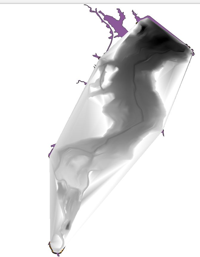
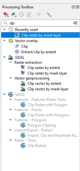
Now that you have your interpolation you may wish to clean it up a bit before moving this file to SAGA. This can be done by navigating over to the toolbar again and typing "clip" into the search bar at the top. This will bring up the "clip raster by mask layer" option. Click that.

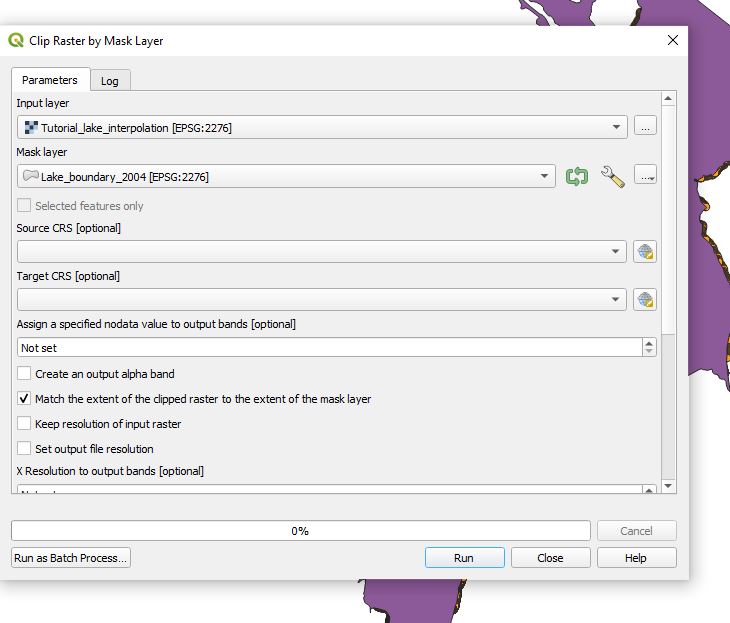
A Text box will have opened after you clicked that option. Select the layer you wish to clip in the input layer (select your interpolation file). Then select the layer that will clip the interpolation under the mask layer. And finally you can make this file also a permanent file by clicking on the three dots beside the clipped (mask) tab near the bottom of the text box.

Now, all you have to do is click "run" and its done!

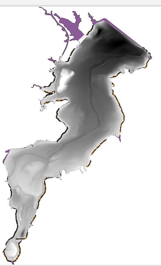
And that is it, you now have done an TIN interpolation of your data and you can move on to the next stage, of moving that data into SAGA.

Determining Overland Flow Distance in SAGA GIS

Once you have SAGA up and running by clicking the icon, we must bring in the DEM we created in the steps prior. To do so go to the modules tab, and follow the "File -> GDAL/OGR -> GDAL: Import Raster" command tree, as in the picture below:

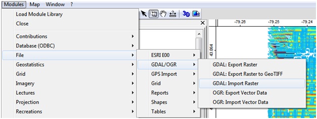
In the window that is brought up, click the load button to bring up a screen where you can navigate to the location of your DEM. Once the location of the DEM has been entered, click okay.

Now that your DEM is displayed on the screen, we begin the steps to determining overland flow distance. This requires us to create the parameters channel network, which in turn requires we create a flow direction map. To create a flow direction map, we must go into "Modules->Terrain Analysis->Preprocessing->Fill Sinks (Wang & Lieu)" as illustrated below:

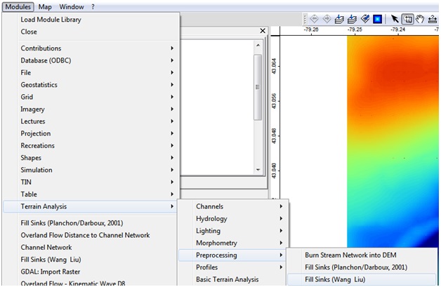
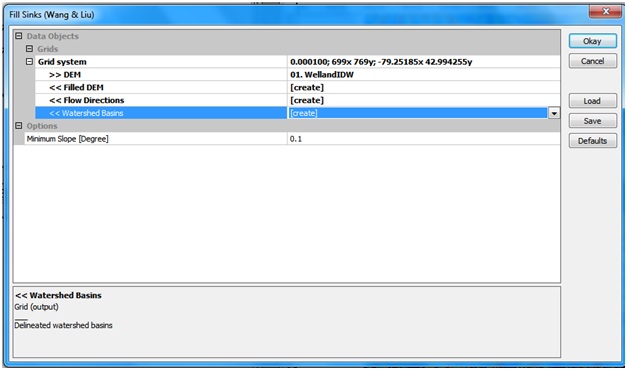
We must use Wang and Lieu method as it is the only one which creates a flow direction map as a method of filling the sink holes within the data. The following screen will appear, in which you must input your original DEM and the grid, while specifying to "create" flow directions, and a filled DEM, such as the following:

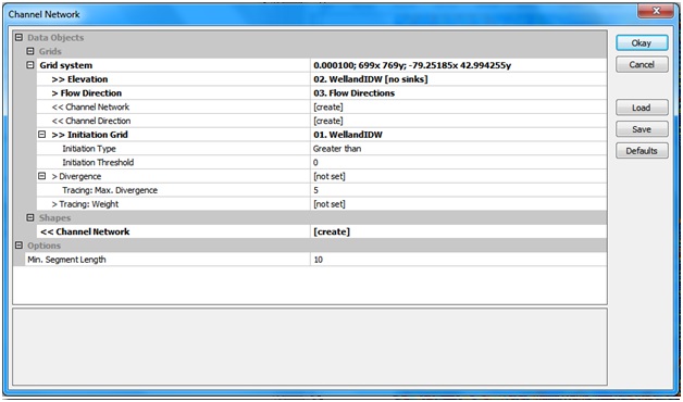
Once we have obtained the flow direction, step 2 of 3 is to determine channel networks via "Modules->Terrain Analysis->Channels->Channel Networks". Once in the dialogue box, be sure to set the grid system to the appropriate system, the Elevation to the filled DEM we just created above, the flow direction to the new flow directions we also just created, and the Initiation Grid to the original DEM. Now, ensuring that channel networks is set to "create", you are free to proceed and press okay. To double check, your screen should look something like the following:

The final step is to Determine the Overland Flow Distance to Channel Network via the Channel Networks and filled DEM we have created above. This tool is located under "Modules->Terrain Analysis->Channels->Overland Flow Distance to Channel Networks", and set your Elevation to the filled DEM, and the Channel Network to the previously created channel network. The rest of the configuration can be adjusted to assess the outputs, but it was found that the default settings yielded the most accurate results. Before proceeding, your window should look something like this:

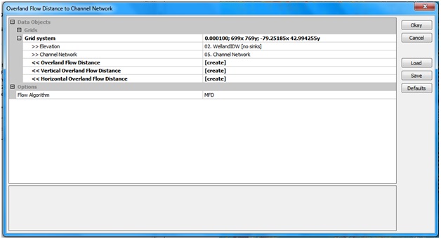
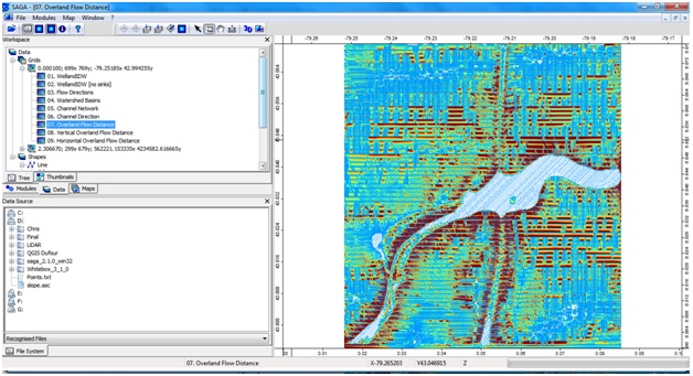
And that's it! Simply click on your new Overland Flow Distance map in the activated data tab and it will appear in the display window as follows:

Conclusions

Due to the relatively low accuracy of the data provided, the results can be interpreted visually from the example provided but not quantitatively. However, this tutorial can be recreated with high resolution LiDAR data given the appropriate time and financial allowances to achieve a much more accurate, analyzable result. The purpose of this wiki was to introduce the user to the interoperability between the two programs and the possibilities each program holds.