Introduction to Vegetation Burn Mapping using Open Data Cube
Contents
Revised Tutorial - 08-10-2022
One of the advantages of open-source software is that it is frequently updated and can often be combined with other open-source software as needed. The caveat is that these softwares are mostly maintained by their creators and contributors, and can sometimes lose that support if these creators and contributors are not available to continue their work. As a result, the instructions in the tutorial below are no longer working. Many packages present version conflicts with other packages, and some are missing whereas when the tutorial was original written, these missing packages were likely installed in tandem with others and didn't require the user to manually install them.
The instructions in the original tutorial below include download a Docker image of Cube-in-a-box. Within that image, there is a file named requirements.txt where additional packages can be added and versions can be specified prior to installation. To give the user a more granular control over software package installation, and a more plastic environment where single packages can be added or removed without having to edit a requirements file and installing all packages again, here you will find instructions to achieve the same workflow using Anaconda instead of Docker.
Initial Setup and Requirements
This tutorial was designed to work on Ubuntu 20.04. The steps below may work on other Linux distributions. However, to ensure there aren't any unexpected behaviours, you should start from an Ubuntu 20.04 workstation or VM.
It is a best practice to run the following commands prior to installing new packages in any Linux distribution. Start by opening a Terminal window with an account that has sudo privileges.
In terminal, type:
sudo apt update -y && sudo apt upgrade -y
Then, you will need some applications to help you in the following steps.
sudo apt install wget git
Datacube Setup
You will need to install Open Data Cube. A tutorial is provided here: https://datacube-core.readthedocs.io/en/latest/installation/setup/ubuntu.html
Following the tutorial, you will need to make a minor change. The ~/.datacube_integration.conf file should be renamed ~/.datacube.conf.
mv ~/.datacube_integration.conf ~/.datacube.conf
Anaconda Setup
Anaconda can be downloaded here: https://www.anaconda.com/products/distribution#Downloads
The following commands will download and install Anaconda 3. These are valid on the date of this revision and may need an updated URL at a future date.
wget https://repo.anaconda.com/archive/Anaconda3-2022.05-Linux-x86_64.sh
sudo bash Anaconda3-2022.05-Linux-x86_64.sh
The Anaconda installation will begin with the license agreement. Follow the steps on screen. Hint: Press space to skip 1 page at a time.
When asked where you want to install Anaconda, it will default to /root/anaconda3/ You should change this path to /opt/anaconda3/
After the installation is complete, you will need to adjust the ownership of that folder and assign it to yourself.
An Example of the command to change ownership will use the username 'sysop' and group name 'sysop'. Typically, your username will be the same as your group name.
sudo chown -R sysop:sysop /opt/anaconda3
Next, we need to initialize Anaconda with these commands:
/opt/anaconda3/bin/conda init
source .bashrc
You will notice that we are now in the base Anaconda environment as indicated by the "(base)" prefix that was added to your command line.
Now we can access the 'conda' command from any location. Let's add the conda-forge channel to Anaconda's package channels.
conda config --add channels conda-forge
Before we set up an environment, we will install a package called nb_conda_kernels that will allow us to select environments from within Jupyter Notebooks.
conda install nb_conda_kernels
To set up an environment, we will use the 'conda create' command with some parameters. We will include the desired version of Python along with some required packages.
conda create -n odc_env python=3.8 datacube ipykernel pandas geopandas matplotlib xarray numpy
This process will take a moment to complete. When it has finished, we can activate the environment we just created using the following command:
conda activate odc_env
You will notice that the base environment indicated by the "(base)" prefix has now changed and we are currently in the odc_env environment.
You can confirm this by verifying that the command line prefix has changed from "(base)" to "(odc_env)".
We can now install more packages that will be required for this workflow. The packages we require are not available through conda or apt, so we will use Python's package manager, pip.
pip install --extra-index-url https://packages.dea.ga.gov.au/ aiobotocore[awcli] boto3==1.24.0 odc-algo odc-ui
Note that specify the version of boto3 to avoid a version compatibility issue that arises from the latest version of boto3 and aiobotocore as they each require a different version of botocore. Using boto3 version 1.24.0 allows us to use a version of botocore that is compatible with aiobotocore as well.
With our dependencies installed, we can now deactivate the odc_env environment and clone the Digital Earth Africa Sandbox Notebooks repository
conda deactivate
git clone https://github.com/digitalearthafrica/deafrica-sandbox-notebooks.git
We need to add the Sentinel 2 dataset into the datacube before we can start using it in the notebook. It can be added using this command:
datacube product add https://explorer.digitalearth.africa/products/s2_l2a.odc-product.yaml
The notebook requires some files in the deafrica_tools, which is located in the Tools folder within the repo we just cloned. Let's move the deafrica_tools folder to the same location as the Burnt_area_mapping notebook that we will be using.
mv deafrica-sandbox-notebooks/Tools/deafrica-tools deafrica-sandbox-notebooks/Real_world_examples/deafrica_tools
Finally, we can run Jupyter Notebooks from the repo folder.
cd deafrica-sandbox-notebooks
jupyter notebook
This will launch into your browser. From there, select the Burnt_area_mapping notebook.
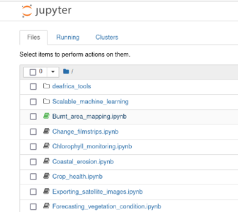
Jupyter Notebook Web GUI. Select the Burnt_area_mapping.ipynb notebook. It will open in a new tab in your browser.

In the new tab, you will see the contents of the Burnt_area_mapping. Before proceeding further, you will need to change the kernel to the conda environment we created, odc_env.
Click on the Kernel menu at the top of the window, then hover over Change Kernel. You can select the conda:odc_env environment from there. Then, you can verify at the top right of the screen that you are using the correct kernel.
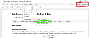
Select the correct kernel from the Kernel menu, and verify that you are using the correct kernel at the top right of the screen. It should match the kernel you select. For this tutorial, this should be the Python[conda env:odc_env] kernel.

From here, you can resume from the Performing Analysis section in the original tutorial below. However, you will find that the datacube query is unable to obtain any data from the Sentinel 2 dataset (s2_l2a). The reason is not yet evident, and further work is required to determine if the query is too restrictive, if the dataset no longer contains this data, or if the syntax needs to change.
Original Tutorial
Introduction to Open Data Cube
In this tutorial the main software framework used is called Open Data Cube (ODC), and its primary function is to make geospatial data management and performing analysis with large amounts of satellite data easier. It offers a complete system for ingesting, managing, and analyzing a wide variety of gridded data through a combination of many python libraries and a PostgreSQL database. It is extremely flexible in that it offers several cloud and local deployment options, can work with multispectral imagery to elevation models and interpolated surfaces and a multitude of ways to interface with the software. This tutorial will be using Jupyter Notebooks to work with ODC, but a web GUI is also available. A great way to think about ODC is like your own personal, open-source Google Earth Engine. However, unlike Google Earth Engine you are in control over the geospatial data and code you create. If you would like to learn more about the ODC framework you can check out the official website here.
Installation Instructions
At first the installation and configuration process for ODC can appear daunting and complex with several dependencies and a long configuration procedure. It is possible to use ODC on Windows, Linux, or macOS, however I find it has the most support and is easiest on Ubuntu. To greatly simplify the installation process ODC has created something called “Cube in a Box”. This is an easy-to-use Docker image that will provide us with a pre-configured reference installation of ODC. Docker uses containerization to package software into units that can be run on most computing environments. More information about Docker and containers can be found here.
Installing Docker
The first step in the installation process will be to install docker.
This tutorial is designed for Ubuntu 20.04 but will likely work on other Linux versions. (Update: on Ubuntu 18.04, try sudo apt install docker docker-compose docker.io)
To install docker run the following command in a new terminal window:
sudo apt-get install docker-compose
And select yes to install any dependencies.
Downloading ODC and Helper Scripts
In this section the Open Data Cube "Cube in a Box" docker configuration will be downloaded from GitHub. Feel free to use the "wget" or "git clone" commands to simplify this process if you undertand how.
Go to:
https://github.com/opendatacube/cube-in-a-box
and download the all the code using the "Download ZIP" button shown in figure one.
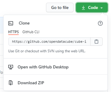
Figure 1: Download button for Github files.

Unzip these files to a desired location in Ubuntu. I chose the downloads folder. This tutorial takes advantage of a number of helper scripts and a code example from Digital Earth Africa.
Go to:
https://github.com/digitalearthafrica/deafrica-sandbox-notebooks
And using the previous download instructions grab the all the code, and extract the .zip file onto your machine.
Next, move the Scripts folder from the Digital Earth Africa folder into the previously-downloaded cube-in-a-box directory's notebooks folder For me I placed Scripts inside /home/admind/Downloads/cube-in-a-box-master/notebooks. Then place the Burnt_area_mapping.ipynb file from the Real_world_examples folder inside deafrica-sandbox-notebooks to the same location as before. This would be /home/admind/Downloads/cube-in-a-box-master/notebooks for me.
The last file is called stac_api_to_dc.py and can be found at:
https://raw.githubusercontent.com/opendatacube/odc-tools/develop/apps/dc_tools/odc/apps/dc_tools/stac_api_to_dc.py
Place this file inside the Scripts folder you just moved. For me this is now /home/admind/Downloads/cube-in-a-box-master/notebooks/Scripts.
At the end your "cube-in-a-box-master/notebooks" folder should look like Figure 2, with 13 python files in the Scripts folder and 3 .ipynb files in the Notebooks folder.
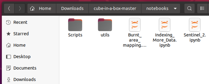
Figure 2: Final location of moved folders and files.

Configuring Cube in a Box
The last step of the installation process is to open terminal from the cube-in-a-box-master folder.
This can be done by right clicking anywhere in the cube-in-a-box-master folder and selecting open in terminal.
After this has been done enter the following command into the terminal window:
sudo docker-compose up
Then after that has completed leave that window open to run and open another terminal with the above process so two terminal windows are open.
In this new terminal enter:
sudo docker-compose exec jupyter datacube -v system init
Then:
sudo docker-compose exec jupyter datacube product add https://raw.githubusercontent.com/digitalearthafrica/config/master/products/esa_s2_l2a.yaml
And finally to make sure it works try:
sudo docker-compose exec jupyter bash -c "stac-to-dc --bbox='25,20,35,30' --collections='sentinel-s2-l2a-cogs' --datetime='2020-01-01/2020-03-31' s2_l2a"
If everything has ran without error messages in the first terminal window with Docker running open an internet browser and go to "localhost".
That is it! You are now ready to move on to the analysis section.
Performing Vegetation Burn Mapping
As stated previously this tutorial uses a code example from Digital Earth Africa that we have already downloaded and installed.
After following the previous instructions you should see Jupyter Notebooks open in the internet browser window.
Importing Geospatial Data
To import the geospatial data for the region that we will be performing analysis on we run the index script.
Open the file named Indexing_More_Data.ipynb in Jupyter Notebooks. Change the fourth line in the first code cell to appear how it does in Figure 3.
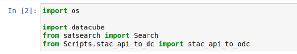
Figure 3: Lines to be changed in first code box.

Next, we will define the location of interest and the time frame. A box is created around the location with the buffer. This can be extended by increasing the buffer value.
Change the second code cell to appear as follows in Figure 4:
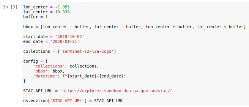
Figure 4: Entering the location and time frame information.

After this run all the cells in order. It should state that approximately 400 items have been indexed.
Performing Analysis
After the indexing has been completed you can close that script and return to the main Jupyter Notebooks directory.
Open the Burnt_area_mapping file. This is a code example created by Digital Earth Africa and contains some instructional material at the beginning and many great code comments to help explain what is happening.
The great part about this example is that it uses the helper scripts to simplify and shorten the code we will be working with. All that we need to do is change the desired parameters throughout the script to get good results. Most of the code blocks are rather self-explanatory and this tutorial will go over ones that are important and/or must be changed.
The analysis will proceed as follows:
- Load packages
- Define location, event date and length for analysis
- Define baseline image
- Create Normalized Burn Ratio Image
- Visualize Burned Area Results
Load packages
Under the description you should see the first code block named "Load Packages"
We need to edit this cell to account for the location in which we placed the helper files. Please add "Scripts." after the word "from" on the last five lines so that the edits appear the same as in figure five.
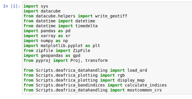
Figure 5: Code to be changed for loading packages.

Define location, event date and length for analysis
We can now run the code cells up until "Select Location". Here we will enter the location chosen for analysis. It can be anywhere in Africa and must be the same location chosen for indexing in the previous step.
See figure six for what this code looks like if you're using the same location as me in Northern Ghana.
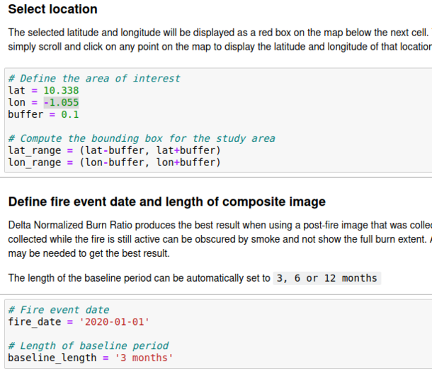
Figure 6. Selecting the location and time of analysis.

We must also enter the data of the fire and length of baseline period from before the fire date to be used. Keep in mind that both these periods must fall within the range of time entered in the indexing data section.
Define baseline image
After the following section has been completed and cells ran we can now run all cells until the "View the selected location" section. Here it will show us a map with boundaries of the area of interest. If this is not showing the correct area it would be good to double check the index coordinates from the previous section.
If the location is correct we can now run the cells in the "Load all baseline data" section. This will run a query of our Sentinel 2 multispectral imagery for the chosen analysis period and select the most clear images using cloud masks. Do not be alarmed if this section takes several minutes to run.
Create Normalized Burn Ratio Image
The Normalized Burn Ratio is an index that can be used to recognize burned areas in images and measure the burn severity. This index calculation is done automatically using the helper scripts. We pass the helper scripts the desired raster data along with our specified parameters and it returns the created Normalized Burn Ratio images.
After running all sections until "Generate Normalized Burn Ratio for baseline period" we can then calculate the burned area in the baseline period before the fire date and again in later cells using the post fire date images. This is done so that we can compare the burned area before and after. Once this section has been ran we can move down a code cell to "Visualise NBR" and our results should appear as follows in Figure 7 if you used the same location and date.
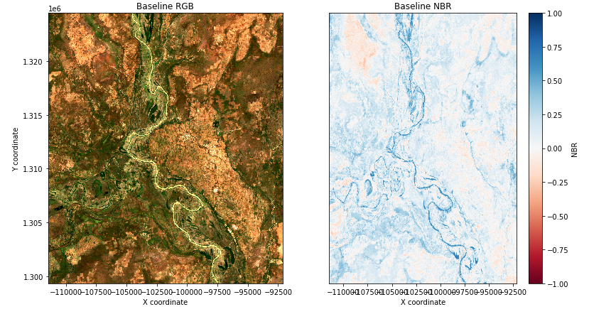
Figure 7. Baseline Normalized Burn Ratio images.

Next, the post fire Normalized Burn Ratio image can be created. Run the code cell under "Load post-fire data" to select the post fire images and "Generate Normalized Burn Ratio for post fire image" to create the post fire Normalized Burn Ratio image.
Visualize Burned Area Results
At this point in the tutorial you can take two options. You can proceed through the following code cells in order while making small changes based on the site, time frame and desired results. This is very technical and will result in you comparing the burned area images previously created with known MODIS fire hotspots, create Delta Normalized Burn Ratio images and calculate the amount of area that was burnt. Or, you can do the simpler option and display the baseline and post fire Normalized Burn Ratio images for a visual comparison. This tutorial is not designed for users with extensive remote sensing knowledge so the simpler option will be shown.
If you skip to the third section from the end titled "Apply threshold to Delta Normalized Burn Ratio" we can display the baseline and post fire Normalized Burn Ratio images. Locate the second, long code block in this section with the first comment "Set up subplots". Run this section and it should provide only four out of six images if you skipped the advanced sections and several error messages. The four images created should appear similar to figure eight. For more information on Normalized Burn Ratio and interpretation check out this helpful explanation.
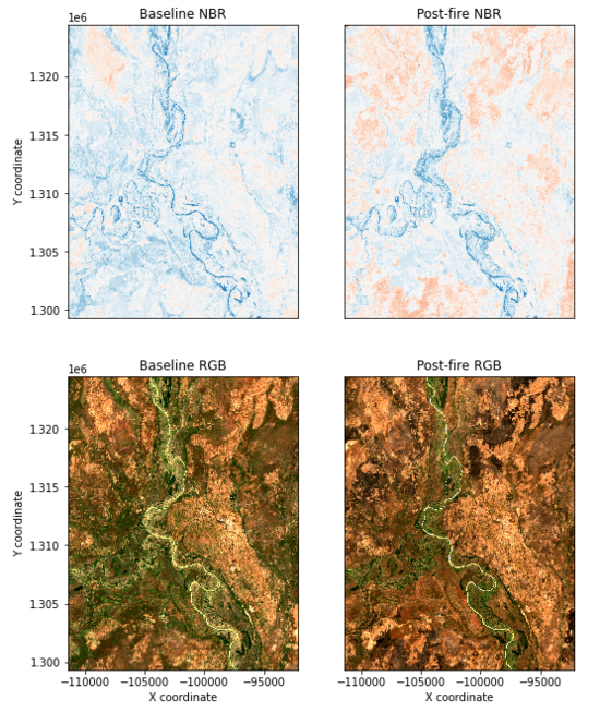
Figure 8. Baseline and post fire Normalized Burn Ratio images.

After the analysis has been completed don't forget to save your results and safely shut down Docker.
In the second terminal window we opened earlier to enter commands we can now enter:
sudo docker-compose down
And a stopped message should now appear in the first terminal running Docker.
Potential Errors
- If you receive an error during package installation like “Hash Sum Mismatch” then make sure you are using the latest version of Oracle VirtualBox. Version 6.1.16 fixes this bug.
- Ambiguous docker errors including “Cannot Connect to daemon” can be resolved by inserting “sudo” infront of the command you are trying to run.
- If you encounter the following error in figure nine when running scripts in Jupyter Notebooks then you must confirm the entire installation process has been followed.
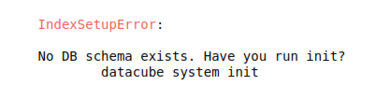
Figure 9. Database Initialization Error.

Sources and Additional Resources
For more information on working with ODC check out the quick Beginner's Guide created by Digital Earth Africa.
Code and Docker Image retrieved from:
- https://github.com/digitalearthafrica/deafrica-sandbox-notebooks
- https://github.com/opendatacube/odc-tools
- https://github.com/opendatacube/cube-in-a-box
Explanation Material and Background Knowledge from: