Land Cover Classification in Google Earth Engine using K-Means (Google Colab)

Land Cover Classification in Google Earth Engine using K-Means (Google Colab)

Author: Muhammad Ba (2025)

Overview

Overview

This tutorial demonstrates how to perform an unsupervised land-cover classification using Google Earth Engine (GEE) and Google Colab. The goal is to transform raw satellite imagery into meaningful land-cover categories by grouping pixels with similar spectral properties.

This classification helps identify water, vegetation, urban areas, and soil patterns across a region. The Ottawa region is used as an example, but the workflow works anywhere in the world. The entire process is cloud-based and does not require installing GIS software.

The workflow uses:

• Sentinel-2 surface reflectance imagery
• K-Means clustering
• Automatic land-cover categorization
• Entirely free, cloud-based tools

This tutorial is suitable for beginners and requires no software installation.

Requirements

Requirements

All tools used in this tutorial are free and accessible from any computer. Google Colab provides a ready-to-use Python environment, while Earth Engine handles all satellite data processing on Google's servers.

Before starting, you need:

• A Google account
• Access to Google Colab: https://colab.research.google.com/
• A Google Earth Engine account: https://earthengine.google.com/signup/

Getting Started in Google Colab

Getting Started in Google Colab

Open a new Colab notebook and run:

!pip install earthengine-api geemap

import ee
import geemap

ee.Authenticate()
ee.Initialize(project='ProjectID')

This installs the Earth Engine API and the geemap visualization library. You must authenticate with your Google account the first time. After that, the notebook connects to Earth Engine and can run geospatial analysis directly from the browser.

Define the Study Area

Define the Study Area

aoi = ee.Geometry.Polygon([
    [
        [-76.35, 45.54],
        [-75.07, 45.54],
        [-75.07, 44.96],
        [-76.35, 44.96],
        [-76.35, 45.54]
    ]
])

The Area of Interest (AOI) defines the region you want to classify. Here we use a rectangular polygon covering part of Ottawa. Earth Engine clips all analysis to this boundary to improve efficiency and ensure clean results.

Load & Visualize Sentinel-2 Imagery

Load & Visualize Sentinel-2 Imagery

s2 = (
    ee.ImageCollection("COPERNICUS/S2_SR_HARMONIZED")
    .filterBounds(aoi)
    .filterDate("2022-06-01", "2022-08-31")
    .filter(ee.Filter.lt('CLOUDY_PIXEL_PERCENTAGE', 20))
)

print("Number of images:", s2.size().getInfo())

median_img = s2.median().clip(aoi)

Visualization:

Map = geemap.Map()
Map.centerObject(aoi, 10)

true_vis = {
    'bands': ['B4', 'B3', 'B2'],
    'min': 0,
    'max': 3000
}

Map.addLayer(median_img, true_vis, "Sentinel-2 True Colour")
Map.addLayer(aoi, {}, "AOI")
Map

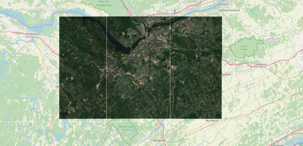
Sentinel-2 imagery provides multispectral reflectance data at 10 to 20 m resolution. The median composite reduces cloud effects and produces a clean, consistent image.

Run K-Means Classification

Run K-Means Classification

n_clusters = 5
bands = ['B2', 'B3', 'B4', 'B8']  # Blue, Green, Red, NIR

training = median_img.select(bands).sample(
    region=aoi,
    scale=10,
    numPixels=5000,
    seed=42
)

clusterer = ee.Clusterer.wekaKMeans(n_clusters).train(training)
classified = median_img.select(bands).cluster(clusterer)

Add the classified layer:

Map.addLayer(classified.randomVisualizer(), {}, "K-Means Classification")
Map

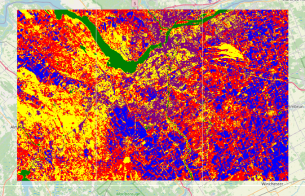
K-Means groups pixels based on their spectral similarity. The output clusters often correspond to broad land-cover categories such as vegetation, soil, water, and urban surfaces.

Exporting Results (Optional)

Exporting Results (Optional)

export = ee.batch.Export.image.toDrive(
    image=classified,
    description='KMeans_Classification',
    folder='GEE_Exports',
    scale=10,
    region=aoi,
    maxPixels=1e13
)
export.start()

Exporting your classification allows you to use the results outside of Earth Engine, such as in QGIS, ArcGIS, or other desktop mapping software. The exported raster keeps the cluster IDs produced by K-Means, which means each pixel will have a numeric value representing its assigned spectral group. Because this is an unsupervised classification, the exported file does not contain labels only cluster numbers. You can manually assign class names later in other software if you wish. Exporting is optional but useful if you want to perform further analysis, create maps, or integrate results into a larger workflow.

Interpreting the Results

Interpreting the Results

K-Means is an unsupervised classification method, which means the algorithm groups pixels based purely on their spectral similarity rather than any real-world meaning. Because of this, the colours used in the visual output are:

• Randomly assigned
• Different every time you run the algorithm
• Not linked to actual land-cover classes

This means that:

• Dark blue is not automatically water
• Green is not guaranteed to be vegetation
• Pink/Red does not always indicate urban areas
• Yellow/Brown may represent dry grass, soil, shadows, or disturbed land

In our example, the “dark blue” cluster represents shadowed vegetation and low-reflectance areas are not water. Since water makes up a small portion of the AOI, those pixels were grouped into a different cluster.

To interpret clusters correctly:

• Compare each cluster with the true-colour Sentinel-2 image
• Focus on spatial patterns instead of colour names
• Remember that K-Means does not understand real-world categories like “urban,” “forest,” or “water”

K-Means produces groups of similar spectral signatures, not ready-made land-cover classes. Meaningful interpretation always requires user comparison with real imagery.

Extending the Tutorial

Extending the Tutorial

Once you complete the basic K-Means workflow, here are some optional extensions you can try to deepen your analysis or build more advanced outputs:

• Try different cluster counts

 Changing the number of clusters (e.g., 3, 5, 7, 10) lets you explore how much detail you want in your land-cover map.

• Add spectral indices to your input data

 Including NDVI, NDMI, or NBR can help the algorithm better distinguish vegetation, moisture, and burned/dry areas.

• Compare land cover across multiple dates

 Try running the classification again for a different year or season to see how the landscape changes over time.

• Export your results to GIS software

 Save the clusters as raster or vector files (GeoJSON/Shapefile) to analyze or edit them further in QGIS or ArcGIS.

• Let users define their own AOI

 Integrate tools such as `Map.draw()` in geemap so users can draw polygons directly on the map.

• Create a simple interpretation table

 Add a small legend describing what each cluster corresponds to (based on your visual comparison with the true-colour image).

These additions are optional but can help tailor the workflow.