Multiple Criteria Evaluation in Allocating Land for Waste Incineration
Contents
Introduction
This tutorial instructs a user in basic, multi-objective decision making using Quantum GIS with Grass and OpenOffice Calc. With it they will be able to import vector and raster data, convert vectors to raster, and use map algebra to produce a land allocation map according to the factors and constraints set up by the project. Since the original time of writing (2010) software capabilities have changed, and the tutorial has been edited to reflect these changes.
Data and Software Versions
The software used for this tutorial are:
QGIS 3.8.3 Zanzibar (https://www.qgis.org/en/site/); and
Apache OpenOffice 4.1.6 (http://www.openoffice.org/).
Note:
Microsoft Excel is also acceptable to complete certain tasks if you wish not to download the Apache OpenOffice Software (Requires minor changes to SQL entries).
Microsoft Excel (https://www.microsoft.com/en-ca/microsoft-365/p/excel/cfq7ttc0k7dx/?activetab=pivot%3aoverviewtab)
While the original version of this tutorial used GRASS GIS, it is not necessary in the current version of QGIS.
Datasets used:
Waterbodies
https://open.ottawa.ca/datasets/water/data
Bedrock (ed. note: There are multiple Datasets of Biophysical Nature in the database, be sure to extract and insert Bedrock dataset only.)
https://library.carleton.ca/find/gis/geospatial-data/national-capital-commission-thematic-data
Landuse 2010 (ed. note: 2010 dataset requires high system capacity as files and datasets are huge. Be sure to use university computers if feasible.)
https://library.carleton.ca/find/gis/geospatial-data/ottawa-thematic-data
Road_Centrelines (Note: Updated versions of Road data can be included in future projects for better outcomes.)
https://open.ottawa.ca/datasets/road-centrelines/explore?location=45.284471%2C-75.687542%2C3.89
QGIS
To begin the project, open QGIS, and perform the following steps:
1. From the browser pane (or the layer tab) add the water, bedrock, and landuse_2005 shapefiles to the project. Note: The Road_centrelines is not needed until the final map is created.
2. If there is a projection conflict, QGIS will generate a popup indicating a transformation. Hit accept. Note: All shapefiles must be reprojected (see below).
To perform the reprojection:
1. Select Vector > Data Management > Reproject layer.
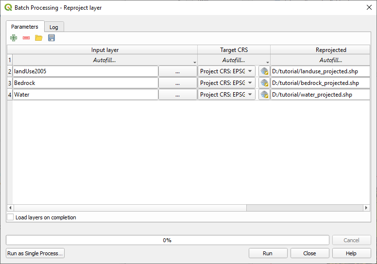
2. Select Run as Batch Process and add the shapefiles as the input layers.
3. Set the project CRS as the Target CRS (should be something similar to NAD83/MTM zone 9).
4. Using the button to the right of the reprojected field name, navigate to the folder containing the other shapefiles.
5.Save each shapefile with a unique name.
6. Ensure Load layers on completion is selected.
7. Run.
An image of this process can be seen in Figure 1.
Figure 1. A screenshot of the batch reprojection tool.
The reprojected shapefiles should load into the project window.
From these reprojected shapefiles, the attribute tables will need to be exported to a CSV exported to the OpenOffice Calc or Microsoft Excel application to facilitate easier editing.
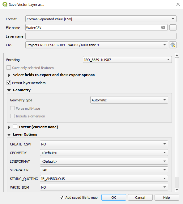
To extract the attribute tables for the shapefiles, right click the layer-> export->save features as->CSV, and apply the relevant parameters, as seen in figure 2.
Figure 2. A screenshot of the Export tool, indicating the parameters required for exportation of the attribute tables in QGIS (Note: The window can change depending on the version of QGIS in use).
Once this step has been completed, the newly created CSVs can be opened in Open Office Calc OR Microsoft Excel.
Feature Value Allocation Using OpenOffice Calc OR Microsoft Excel
To determine the parcels of land most suitable for Waste Depots and Incineration Sites we can assign a specific cost value to acceptable and unacceptable attributes. Preparing the vector data in this manner will allow us to easily determine the placement of sites by visual inspection.
A) Feature Value Allocation: Landuse
The land use data categorizes parcels of land according to Ottawa municipal guidelines. Acceptable land use categories for this project are:
- Vacant Land
- Vacant Building
- Idle and Shrub Land
- Open Space
- Pits and Quarries
Industrial Areas can also be used in the land allocation although in accordance with the definition of industrial Area by the City of Ottawa, Industrial Areas are places of manufacturing, assembly, warehousing or storage and wholesaling of goods. Nonetheless, they can release many harmful gases and chemicals causing possible effects on public living around it. Therefore, they have not been included in the updated version of the study to take into consideration any harm that they may cause.
All other land use categories are unacceptable. Acceptable categories will receive a low cost value and unacceptable categories will receive a high cost value. In order to do this we can use OpenOffice Calc or Microsoft Excel program to modify the attribute files. Although this procedure can be done using GRASS, OpenOffice Calc and Excel consumes fewer system resources to perform the same operation because it is not concerned with the spatial component of the vector data using the database.
Note: Majority of the steps can be replicated in Microsoft Excel. Instructions are added in areas where changes in SQL entries are required.
B)Importing and Toggling Data in OpenOffice Calc
1.To begin allocation, activate the OpenOffice Calc program and open the Landuse_2010 CSV.
2. A “character set encoding” dialogue box will appear. Note that some of the accented characters may not convert correctly, even if the encoding language is identical; this can be edited using the “find and replace” function. Be sure to select "TAB" as the separator, as shown in figure 3.
Figure 5. OpenOffice Calc character set encoding.
Now that the Landuse database file has been loaded into the spreadsheet:
1.create a column named "Value".
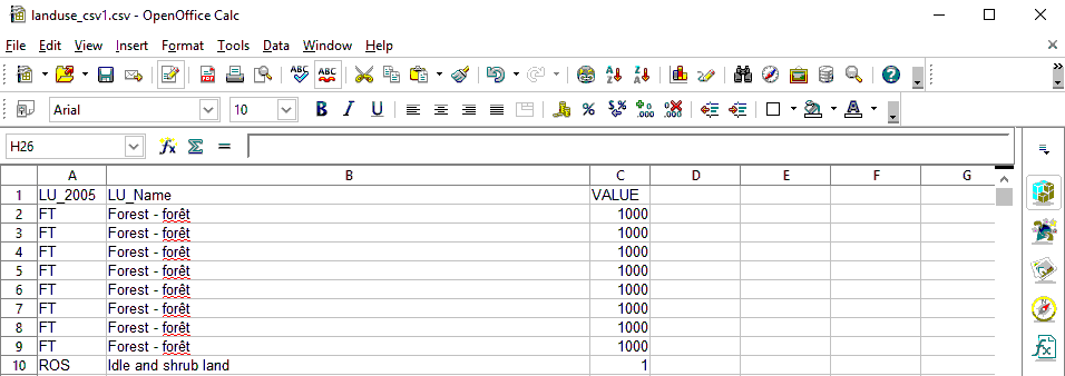
2. To assign the proper cost values to the categories we can use a logical function that will assign “1” to acceptable categories and “1000” to unacceptable categories. In the VALUE column, type =IF(A2="V1"; 1; IF(A2="M1"; 1; IF(A2="V2"; 1; IF(A2="ROS"; 1; IF(A2="OS"; 1; IF(A2="QS"; 1; 1000))))). This will sort the LU_2005 values for later processing.
3. Apply this formula to the entire column by selecting the small black box in the right-hand corner and dragging it down the column. See figure 6.
Figure 6. A sample of the Landuse_2005 edited CSV.
4. Save the file, and select “Keep Current Format” when prompted.
C) Feature Value Allocation: Bedrock
The bedrock data contains bedrock composition and is limited to the Ottawa-Central region. We want to allocate land upon bedrock with little to no remaining economic value to other industries or to the City of Ottawa. According to the geological survey carried out by the Ministry of Natural Resources’ Mineral Resource division the Ottawa-Central region describes several bedrock types of little to no economic value:
- EASTVIEW FORMATION, DARK GREY LIMESTONE WITH SHALE BANDS
- MARCH FORMATION, INTERBEDED GREY CALCAREOUS SANDSTONE & DOLOMITE.
- CARLSBAD FORMATION, GREY SHALE SOME DOLOMITE LAYERS.
- BILLINGS FORMATION
- ROCKCLIFFE FORMATION, GREY GREEN SHALE WITH GREY SANDSTONE LENSES.
- QUATERNARY FORMATION, THICK DRIFT, RECENT ALLUVIUM & PLEISTOCENE GLACIAL DEPOSITS.
Report the same steps as the landuse_2005 allocation above, using the formula =IF(C2=1; 1; IF(C2=2; 1; IF(C2=4; 1; IF(C2=5; 1; IF(C2=10; 1; IF(C2=12; 1; 1000)))))), which uses the "class" values to sort the data.
D) Feature Value Allocation: Water
The water polygon vector contains data on all water features in the Ottawa region, including rivers, streams, and ponds. For this project, all water features will receive a high cost value of 1000. Under the VALUE column, use the formula =1000, and apply to the entire column.
E) Importing and Toggling Data in Microsoft Excel
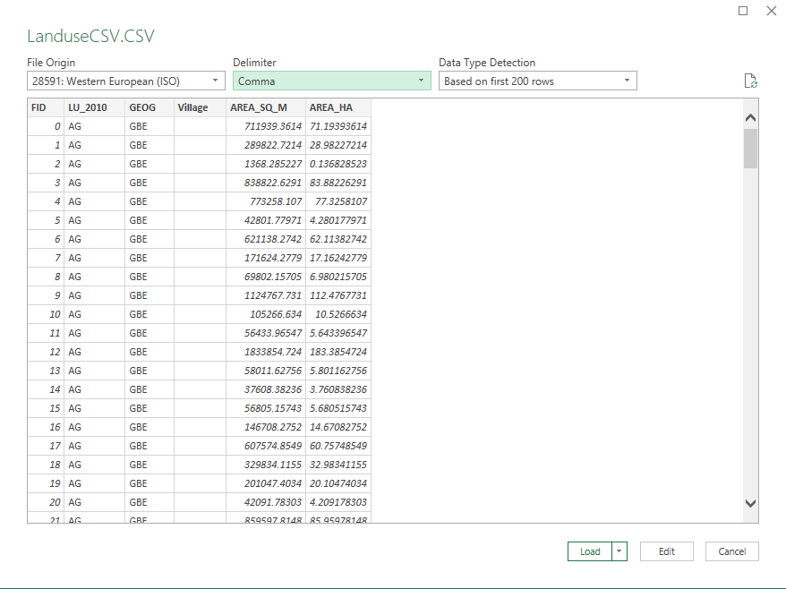
1. To begin allocation using Microsoft Excel, you need to import the data in a specific format. Open Excel ---> Data ---> Get Data ---> From File ---> From CSV/File
2. A window pane similar to the Figure Below will appear. Change and toggle the delimiter to get results similar to the figure below. Load the data after.
Figure 3: Data import pane in microsoft Excel.
3. Once the data is loaded, Add a new Field into the top column named 'Value'. In the first cell, Add the following SQL entry for each file-
Landuse CSV: "=IF(A3="V1",1,IF(A3="V2",1,IF(A3="ROS",1,IF(A3="OS",1,IF(A3="QS",1,1000)))))"
Bedrock CSV: "=IF(C3=1, 3, IF(C3=5, 1, IF(C3=8, 1, IF(C3=9, 1, IF(C3=10, 1, IF(C3=12, 1, 1000))))))"
Water CSV: Follow the same steps as mentioned in OpenOffice Calc section above.
4. With entry of each cell, the remaining cells in the workbook should be completed automatically.
Figure 4: How to input the SQL entry in Microsoft Excel.
Joining Attributes In QGIS
Once the CSVs are complete, they need to be added to QGIS, and joined to the respective shapefiles. To add them:
Step 1.Navigate to the layer tab--> add layer--> add delimited text layer. A popup will appear, and the parameters can be set.
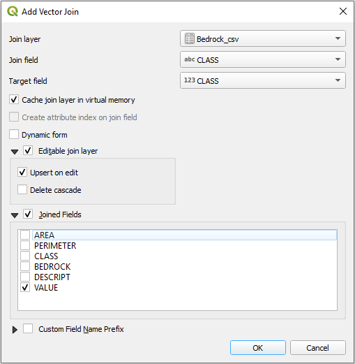
Step 2. For the join, Right click the target shapefile -> properties -> joins -> add joins (indicated in this version as a plus sign near the bottom of the window)-> select the target csv -> input parameters. Step 3. Ensure the join field and target field are the same, the editable join layer is toggled, and the selected joined field is "VALUE". An example can be seen in figure 7.
Figure 7. An example of the join function.
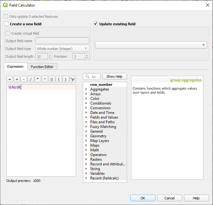
Step 4. To ensure the “VALUE” attribute is an integer, not a string, open the attribute table of each shapefile, select the edit button, add a new integer field with a length of 4, and use field calculator to copy the string field(see figure 8) by:
1. Select the “update field” button;
2. Type in the string field name;
3. Select okay.
Figure 8. An example of the field calculator function.
Converting Vector Data to Raster
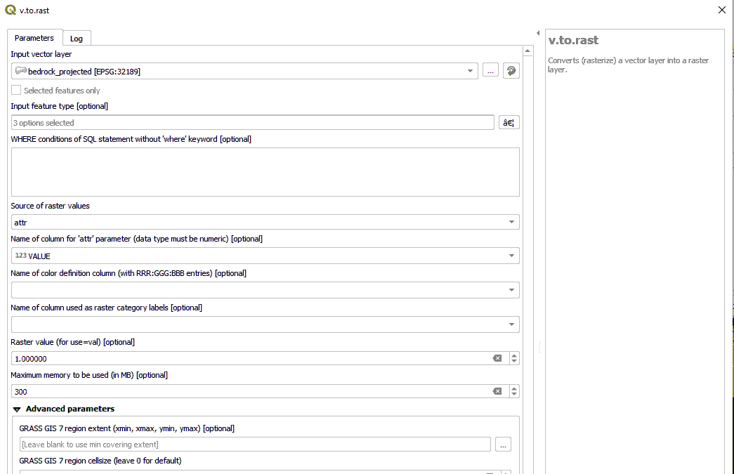
Once the CSVs have been joined to the shapefiles, they can be converted from vector to raster, as shown in figure 9.
1. Navigate to the processing toolbox--> GRASS-->Vector-->v.to.rast.
2. Set the source of raster values to "attr" parameter, the "VALUE" column as the "attr" parameter, and the region cell size as 25. Name the raster appropriately,
3. run.
Figure 9. A screenshot of the vector to raster tool.
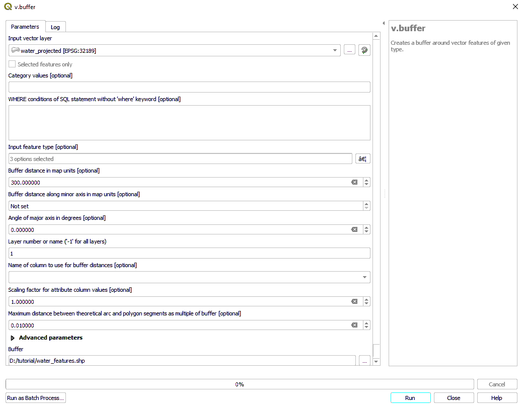
Before we convert the Water vector to raster we must apply a buffer to it. No Incineration Facility or Waste Depot should be constructed within 300 metres of any body of water. To do this:
1. Navigate to the tool by Processing toolbox--> Vector--> v.buffer (as seen in figure 10).
2. Set the buffer distance in map units to "300", and name the shapefile appropriately.
3. All other parameters can be left as the default.
4. Run.
Once this has completed, the buffed water features can be rasterized, as outlined above.
Figure 10. An example of the "vector buffer" tool.
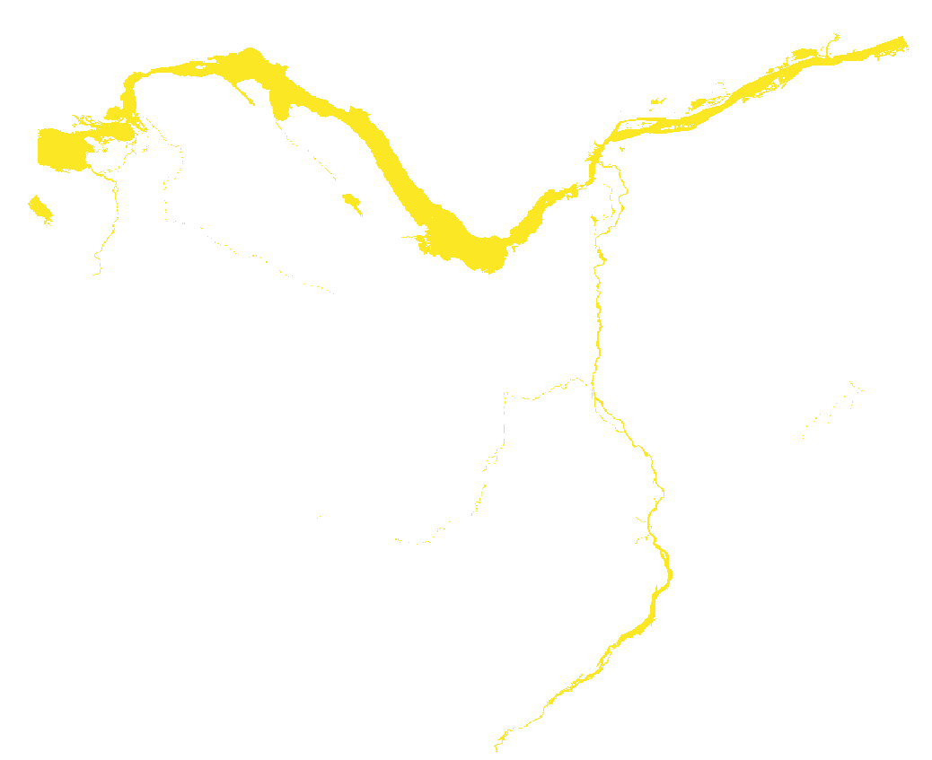
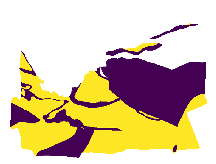
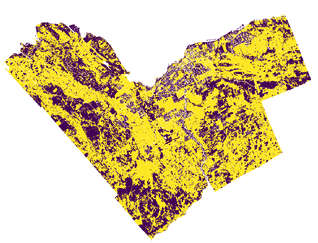
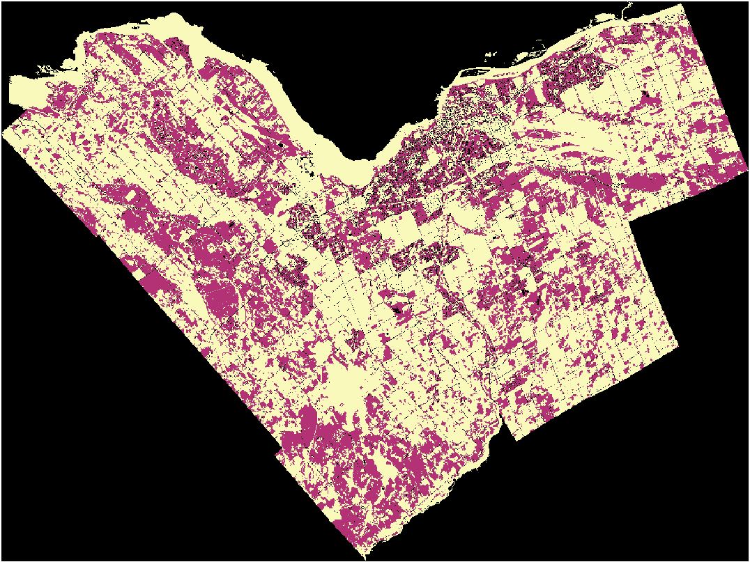
Now that there are three rasters, Open the layer properties of each and navigate to symbology, and hit the classify button to bring the pixel count down to 1 and/or 1000 for the raster files. The results can be seen in the below figures. Yellow shoes areas of high cost (unsuitable) and purple show the areas of low cost (suitable).
Figure 11. The result of rasterization on the buffed water data.
Figure 12. The result of rasterization on the bedrock data.
Figure 13. The result of rasterization on the landuse data.
Using Map Algebra to Allocate Best Area for Incineration
Now that we have the 3 rasters, we can create a Land Use Suitability Map. This map should indicate the maximum area for use by incineration facilities and waste depots.
To create the map:
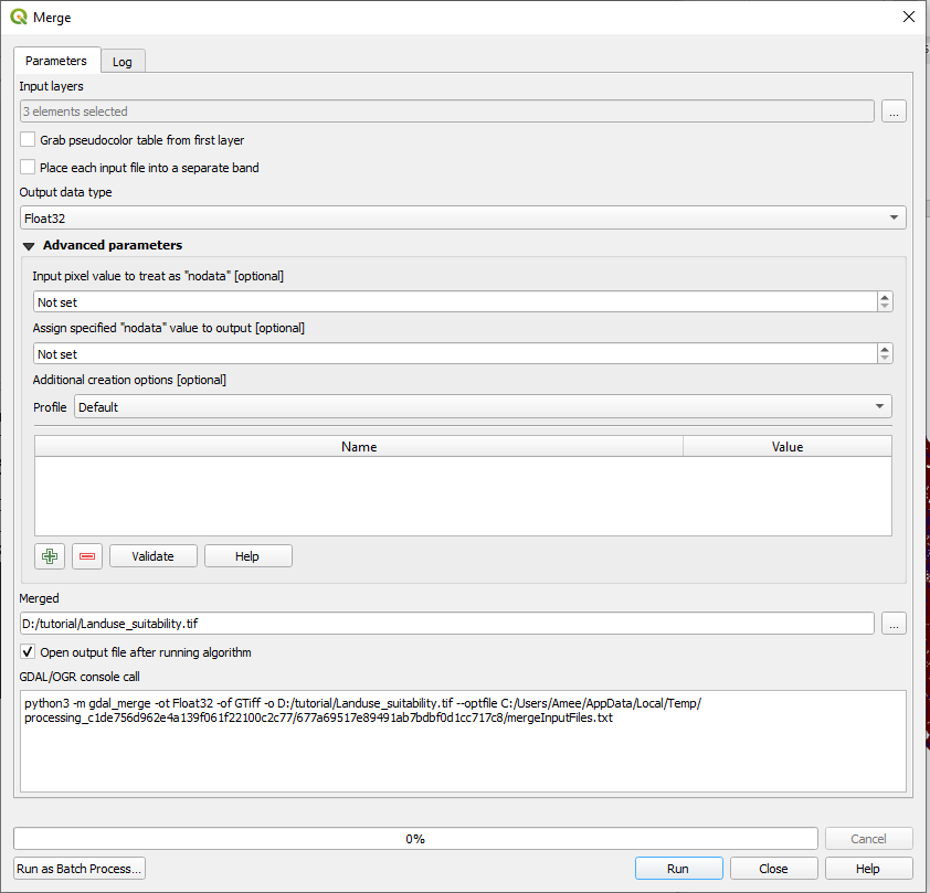
1. From the raster tab, navigate to miscellaneous, then merge. An example of the tool can be seen in figure 14.
2. Add all three rasters to the input layers.
3. Leave the defaults.
4. Name the file appropriately.
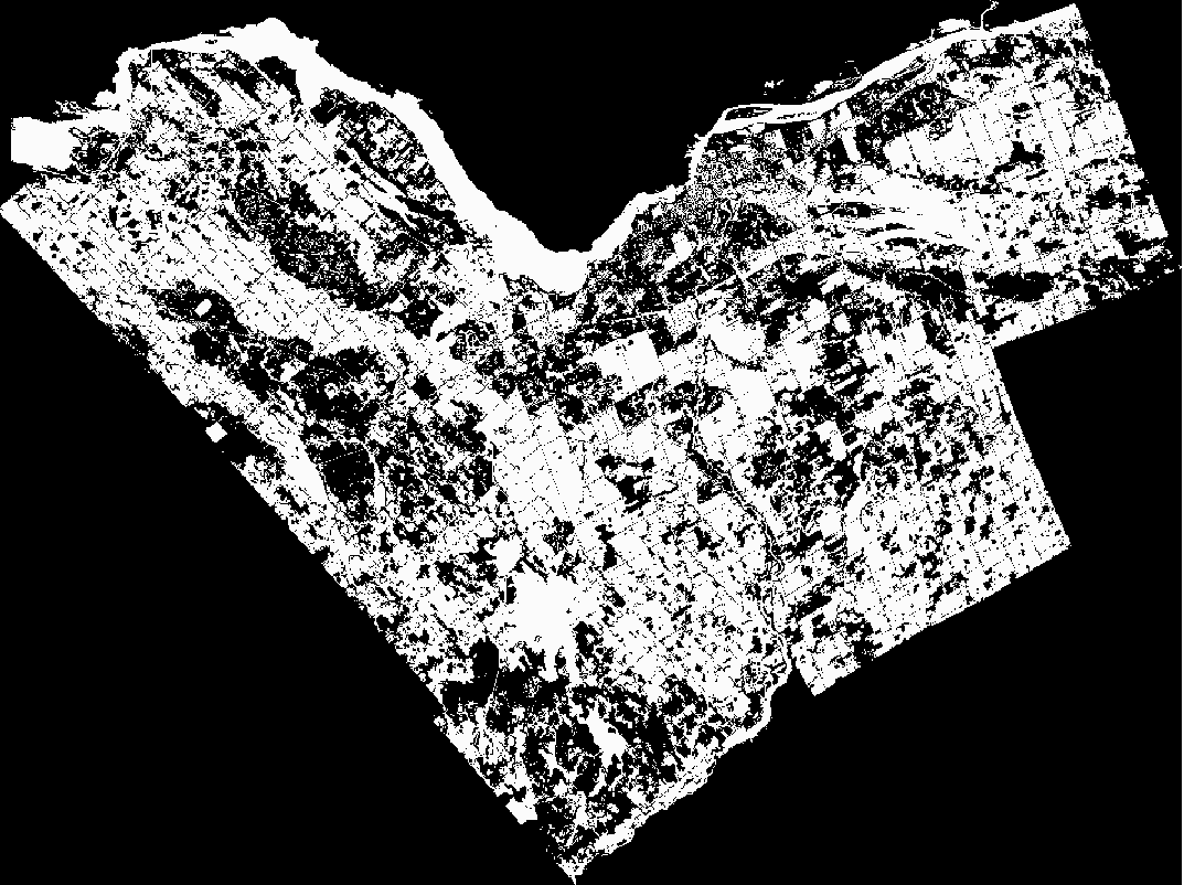
5. Run. Figure 15 is an example of the original output.
Figure 14. A screenshot of the merge tool.
Figure 15. The original output of the "merge" tool.
As seen in figure 15, the original output is black and white, and only has two values; 0 and 1000. This can be adjusted by changing the symbology to paletted/Unique values, selecting the "classify" button, and it will render the raster to 0, 1, and 1000 values. The result can be seen in figure 15.
Figure 16.Land suitability.
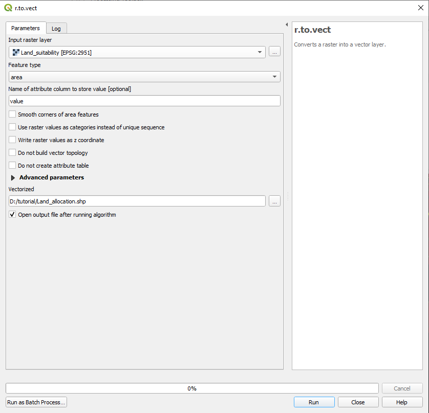
The final step is to reconvert the raster to vector, and add the road_centerlines data. To reconvert:
1. navigate to Processing Toolbox--> GRASS--> Raster--> r.to.vect.
2. Set the input as the land suitability raster, with "area" as the feature type.
3. Name appropriately.
4. Leave the rest as default.
5. Run.
Figure 17. The "raster to vector" tool.
It is here that the road_centerlines become relevant, so if they are not on the mapset yet, they can be added now.
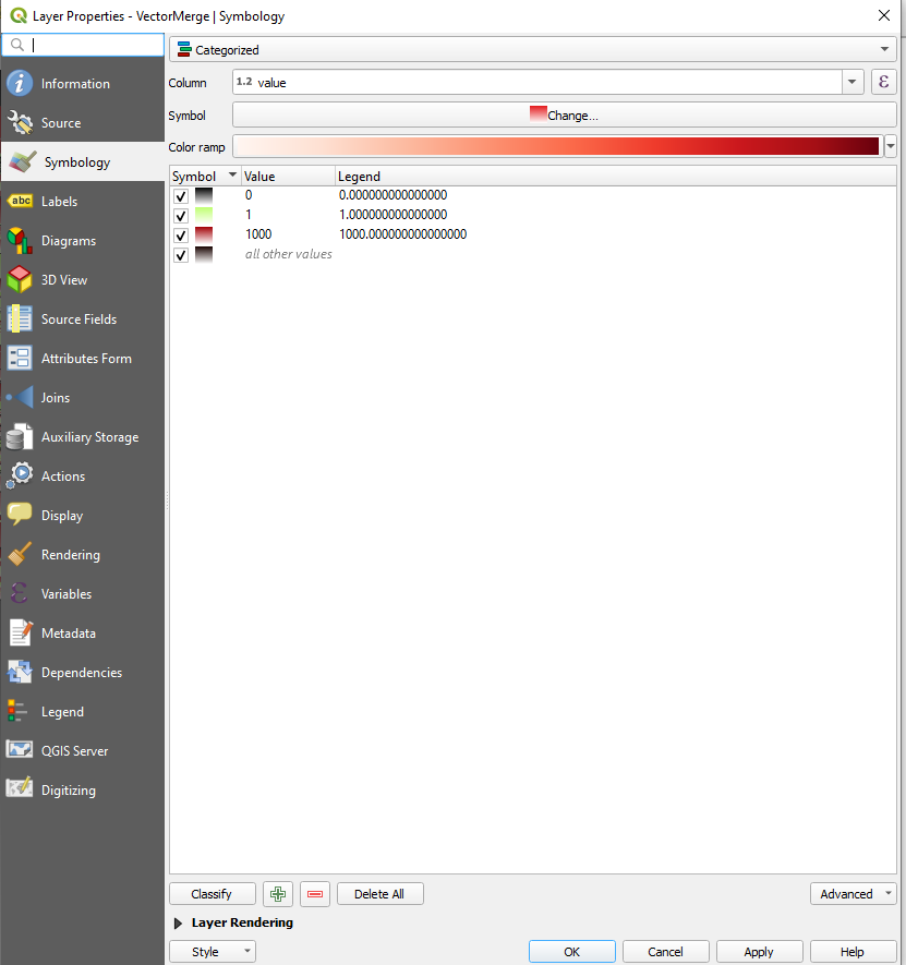
Open the symbology settings by right-clicking the vector and selecting “Properties”.
In the “symbology” tab, set the Legend Type to “Catagorized” and Classification field (here labelled "column") to “VALUE”, and click the Classify radio button. This should add the "0", "1", and "1000" values.
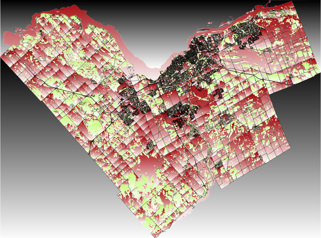
Figure 18. The symbology of the newly created vector map should indicate the null values (represented by the 0), the "1"(indicating suitability) and the "1000" (indicating unsuitability), shown here in grey, green, and red, respectively. The road network is indicated in black."
Figure 19. A land allocation map with Green areas displaying possible Waste Incineration Facility Locations.
If desired, a map layout can be applied, but it is not strictly necessary.
Conclusion
This tutorial showed how to create a land allocation map for waste allocation, using two open-source software packages. The original version of the project included steps that required coding, as well as the use of a stand-alone GRASS GIS application. In the updated version of QGIS integrated with GRASS, this is no longer necessary. However, QGIS does have command prompt scripting capabilities, if a person preferred. OpenOffice Calc is an open source, MS Excel alternative that enables editing of the attribute tables. Ms Excel can be used for users that find it easier to use and execute similar activites. It is possible to perform this task within QGIS itself using the map calculator in the application, but this option can be less intuitive, and more cumbersome.
References
- Fraser, John Z. (1976). Mineral Resource Survey. In DIVISION OF MINES, GEOLOGICAL BRANCH Open File Report 5217. Retried November 25, 2010 from
