Random Forest (ViGrA) Classification in SAGA

Tutorial on preforming Random Forest Classification using R

Purpose

This tutorial will demonstrate how to perform a Random Forest classification using the ViGrA tool found in SAGA. Random Forest (RF) is an algorithm that uses an ensemble of decision trees. Using multiple decision trees, the highest probability tree can be used to perform a classification or regression. This tutorial will cover the basics of creating training data, and running a land cover Random Forest classification in SAGA.

Introduction

Random Forest (RF) classification is an ensemble learning method, which uses decision tree classifiers. Where a random sub-sample of the data is taken and a classification is made from that sub-sample. This process is done to a user-specified amount of runs and the average is taken to improve accuracy and prevent over-fitting. There is no better algorithm for classification, it runs efficiently on large data bases and even with large amount of variables (100+). It provides unbiased estimates and the tree provides a visual representation of which classes are important and which ones are not. Also, it allows for easy computation of similarities and differences between variables and also statistical uncertainty for classification. Furthermore, a basic Random Forest imagine classification is available in the open access software SAGA using the ViGrA.

Further information on Random Forest can be found at wikipedia.org. Random Forest

Software

The Random Forest classification can be run in a program as a script such as R or Python. However, these programs can have a steep learning curve and be complex with importing and exporting files. Luckily SAGA version 2.1.2 contains a Random Forest Classification tool that uses ViGrA. Note: Older version 2.0.8 of SAGA does not contain the Random Forest Classification (ViGrA) tool.

Data

There are two types of data required to perform a supervised random forest classification; variables and a training data set.

-The variables used for a classification are raster images. These variables include spectrum wavelength image bands such as (Red, Green, Blue and Near Infrared), temperature, and Digital Elevation models (DEMs), and determined derivatives such as (slope and aspect). Other variables can be used such as vector and table data, but these options are not explored in this tutorial.

-Training data is a data set that has to be a polygon layer for the tool. Training data is usually represented as a point or polygon, and these points or polygons refer to a specific class. A class is a unique feature or trait that is represented in a classification, they are created to illustrate locations and patterns. The training data has to be created manually and is often time consuming, as the large the training data sets have to be visually determined for each point or polygon. The larger the training data set, the better spatial representation of the area, and the greater the variability in random sample selection, which both increase the classification accuracy. If your training data is in a point format then it can be easily buffered to create a small polygon that can be used.

Tutorial for Random Forest Classification (ViGrA)

Uploading information into SAGA

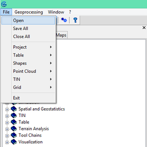
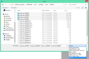
To upload files into SAGA, use your mouse and go to File->Open, from here a load screen will appear, click on the bottom right corner of the screen and select the all files tab, select your files and click open

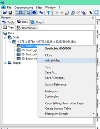
To visualize your data, select the data you would like to display and click on Add to Map

Creating Training Data (Points) for each class

To create training data, the overall data set has to contain a minimum of 100 random points. We will create three classes of point files for the classification of three classes (water, forest, and urban). The water class will be demonstrated below. Note: that the forest and urban classes are created in the same fashion.

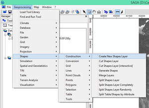
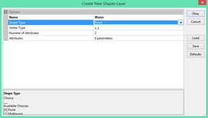
To create a point file, we start by creating a new layer file. Select geoprocessing-> Shapes-> add new shape file

Name your class for points and make sure the shape type is selected to be points.

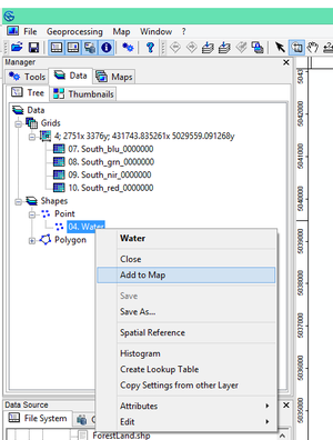
A point layer file has been created. Now we must add the points. To add a point right click on the created layer and add to map to ensure that the layer has been activated.

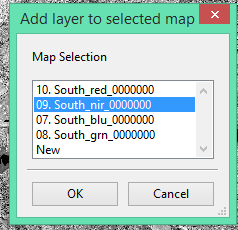
You will see a small screen asking which map to upload the shape file to. As I will be creating a class for water I will select the image band that best represent this class, in this case the NIR band represents water in a black.

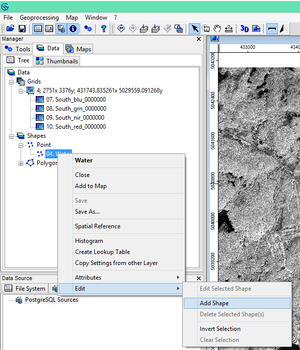
To add a point activate the add shape feature that is in the Edit-->Add Shape

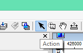
Now that the shape file add has been activated, we can create a point file by selecting the action tool in the bar

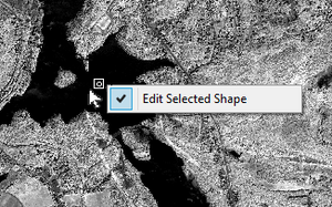
Then select the area in which you wish to create the point and click. A small square with a circle inside will form, that represents the location that you chose. To finalize the creation either press enter or double left click on the mouse and click on the only option to edit selected shapes.

Repeat the add shape process for the water layer file to keep adding points to the layer. Add enough points that will allow you to properly sample the area. I would recommend a minimum of 30 points per class.

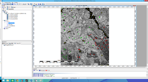
You should have a training data set now of points that resembles the following image.

Once your training data has been created for a class repeat the same process to create a new layer file for each class you will be using for your classification.

Buffering and Merging layers

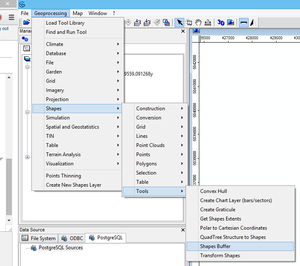
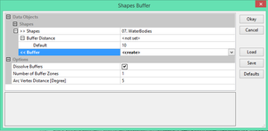
The points need to be converted into polygons, which is achieved by buffering the points. Points have to be individually buffered before they are merged. To buffer a point file select Shapes-> Tasks-> Shapes buffer

In the menu that pops up, select the buffer distance to 'not set' and then select a appropriate buffer size. I chose 10 for my classification. The greater detail your training data is, the smaller the size you can select. Or, if the features are very similar you can choose a larger buffer size.

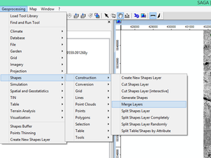
Once you have created the three buffer files, you can merge these polygons together to create a single data set of polygons for your classification training data. To merge layers select the Shapes->Construction->Merge Layers

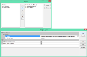
Then you have to select the layers you wish to merge (making sure they are the buffer layers).

You will have your overall polygon training data set to be used in your classification. NOTE: you should have a smaller cross validation data set created as well following the same steps however only using 25-30% of your total points.

Running a random forest classification

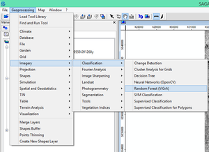
We will be using the Random Forest Classification (ViGrA) tool to perform a supervised classification. To open the tool select the following options Imagery->Classification->Random Forest (ViGrA)

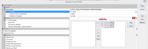
Then upload all the image bands you wish to load by selecting the Grid system you wish to use, and then the Features you wish to upload.

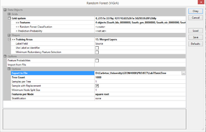
Select the number of trees you wish to create and other settings. Note: that running 1000 trees took approximately 3 mins to run on a higher end PC(intel i7-4790K 4.00 quad core processor). Refrain from running larger trees then this unless you are allowing it to run overnight. The following are the settings that I have set up as, there is little documentation on some of these settings.

Data Objects

Grid

Grid system -> Selects which grid system to load for you to upload your variables
>>Features -> Select which features you wish to upload into your variables
<<Random Forest classification -> select create to create a new grid, or overwrite a existing one
<Prediction Probability -> Select the create to create a new grid for each class specifically 

Shapes

>> Training Areas -> Select the merged buffer training data that you will be using
 Label Field -> Sets which attribute header you will be using for the classification (recommend not set)   
 Use Label as Identifier -> allows you to decide if you will be using the header of the file as the class (leave uncheck if unsure)
 The Minimum Redundancy Feature Selection -> Unsure of its purpose for the classification. More information can be found here on it. mRMR 

Options

Feature Probabilities -> Unsure of its purpose
Import from file -> if a previous Random forest classification has been performed the tree and settings can be loaded here

-Options

 Export to File -> this will export your decision tree and settings as a file to be loaded on a later classification
 Tree count -> this is how many trees you wish to create (note try to remain below 1000 as more can cause slow classification)
 Samples per Tree - > This will specify the fraction of total number of samples to be used per tree for learning.
 Sample with replacement -> Checking this box improves randomness as it will sample the training data with replacement.
 Minimum Node Split Size -> This will allow the tool to know how many samples are require to make a split, use 1 to use all samples and complete growth  
 Features to Node -> Unsure remained default at square root
 Stratification -> Unsure remained default at none

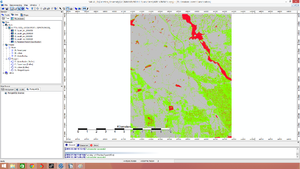
After the classification has been produced the final image is displayed and may result in visually displeasing colours as they are produced at random.

Validation

There are many types of validation for classification. One method for validation of random forest is to use a small sample of your training data (30%), and perform a random forest classification on this data following the same steps described in this tutorial and compare it to your actual random forest classification. There are many ways to perform a validation, and they will not be covered here as it is not included in the tool and would be broken into mulitple tutorials.

How to edit class colours

How to change the colours in a map for better visual representation.

Now that you have successfully performed a Random Forest Classification, the output maps colour is displeasing.

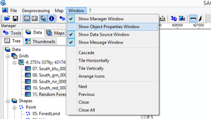
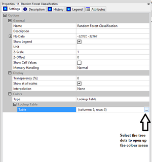
To change the properties of a map we must ensure that the properties tab is activated. to activate the properties tab click on the window tab and select the show properties

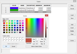
Then choose the lookup table options

From here change the colours into your desired format

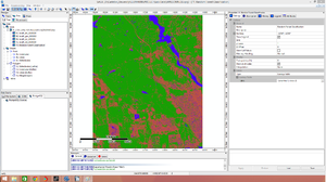
Then you will have your final product

Conclusion

Overall, the tool works well and can successfully produce a classification. Although it may be limited in the speed of its execution, the user does not need to have knowledge of scripting to run a classification. With its lack of documentation and explanation, only users that have performed a RFC before may understand how to use the tool, before this tutorial was created of course. However, the largest downfall of the tool is exclusion of the decision tree that is used to make the classification. This tree provides a visual representation of which classes are important and which ones are not and is one of the greatest strengths of performing a RFC. Therefore, the tool may run a successful RFC, but it looses the strength of RF.

References

SAGA software - http://www.saga-gis.org/en/index.html

ViGrA website - http://ukoethe.github.io/vigra/

Variables for IKONOS satellite images in the Blue,Green, Red and Near Infrared bands in Southern Gatineau Park. Provided by Murray Richardson