Social Spatial Network (SSN) Creation and Analysis using SNoMaN Web App
Contents
Introduction to Social Spatial Networks (SSNs):
Researchers in the social sciences have used social networks/sociograms to visualize the connections and relationships of people in a community since the 1930s (Andris & Sarkar, 2022). However, these networks are aspatial and do not integrate geospatial information about individuals to analyze and explain these relationships (and lack of relationships). Based on Tobler's First Law (Tobler, 1970) "everything is related to everything else, but near things are more related than distant things", it could be theorized that people who live/work near one another are more likely to have similar characteristics and to interact more frequently, but this cannot be confirmed using sociograms alone as they lack a spatial component. Networking and graph theory from the field of Computer Science is also tangentially related to social-spatial networking, but is generally focused on the abstract or theoretical connections between nodes, rather than simulations of real world phenomena (Bondy, 1982). Finally, network analysis also exists within traditional GIS fields and discussions, though this generally based on the distribution of goods and services along pre-defined road/stream networks, rather than a focus on the relationship/connection outside of pre-defined networks (Andris & Sarkar, 2022). Social-Spatial Networks are an integration of the ideas found in these different fields to analyze and document social relationships/connections between individuals situated within their geospatial locations to better understand how connections are formed and maintained.
Term Definitions
In Social-Spatial Network analysis, Nodes are specific geolocated points representing people, businesses, or other points of interest. All nodes need at minimum two datapoints, a unique name/ID to reference the node and some form of location information that can be converted into a (lat, long) pair. Nodes may also contain auxiliary information about the point being represented, such as demographic information on a participant, or classifications of a business type.
Edges represent a social connection between two nodes and are at minimum composed of a pair of names/IDs that are found in the node list, all names within the edge list must be found exactly in the node list, or the program may crash. Similarly to nodes, edges can also contain additional information about a connection, such as a strength value or a type classification that may be used to weight the algorithms.
Buidling a Dataset for a Social-Spatial Network:
For the purposes of this tutorial we will use a mock dataset created from the personal knowledge of this tutorial writer about the characters of the audio-fiction podcast, The Magnus Archives, produced by Rusty Quill under a Creative Commons Attribution-NonCommercial-ShareAlike 4.0 International License. Non-specific location information for the nodes was taken from the Magnus Archives Wikia as well as a fan-made map (found here) for some that were unclear, alongside my own knowledge of the plot/characters when ambiguous/multiple locations. The dataset is available to download from the writer’s Github account https://github.com/otter-lights/SSN-Dataset_TheMagnusArchives and is composed of four files, the initial nodes.csv file and the accompanying location.csv file, which are used to create a final geolocated nodes.csv file, as well as an edges.csv file.
Define Your Nodes

The first step to creating a social spatial networking dataset is to define the sample that will make up your nodes. Depending on the project this may be a previously defined set of participants, but often the scope of the node definition needs to be determined. Since the Magnus Archives dataset was made for this tutorial rather than actual research characters were selected to be included without considerable thought or planning, but in real-life scenarios a more systematic approach should generally be used.
Initial data creation was done in a spreadsheet software, chosen characters were listed alongside their in-universe affiliation and a written description of their main location. Character names are going to be used as the node identifier so they must be unique within the dataset, affiliations and locations can have duplication.
Geolocation of Written Descriptions
The next step to create the node list is to turn the written location descriptions identified previously and geolocate them to a latitude and longitude pair. First this required a list of all unique location descriptions in the original file, for a smaller datasets this can be done manually; however, for larger datasets or datasets with a lot of duplication, scraping of unique descriptions can be done in R. Code for this is shown in Figure 2 below.


After the unique descriptions have been saved into a 'unique_locs.csv' file, the "real_loc" column can be filled out with more specific real world locations that are determined after the fact, such as street addresses or coordinate points, as seen in Figure 3 above. This column will be used as the input for geolocation using OpenStreetMaps. Coordinate pairs being used as real locations should be in decimal degrees as single column with a comma separator and no quotes or other formatting. This .csv file can then be reimported into your R script.
The final step to creating the node list for SSN analysis is to geolocate each of these real-world locations and match them to their corresponding nodes, using the code shown in Figure 4. Geolocation is done using the "tmaptools" library, specifically the "geocode_OSM(query, return.first.only = TRUE, details = FALSE, as.data.frame = TRUE)" function. This line of code will take the query provided, in this case an iteration of through each row of real_locs, and query the OpenStreetMap Nominatim server, returning only the first result as a dataframe. Details about the type of OSM feature can be included in the query results if details = TRUE in the function parameters, this can be used for verification and troubleshooting for weirdly placed points, but is not included in this workflow. The lat,lon pairs from these query results are saved alongside the unique locations and then matched to the original nodes using another for loop, and the final node list can be saved to a .csv file, that should now include (at minimum) columns for a unique identifier, lat, and long.
Relationship Definitions
The last element of dataset creation for social-spatial networking is to identify and define the relationships between the nodes/participants. This can be done in a number of ways depending on the density of the network and the number of edges needed to be recorded. For this use-case, all possible edges between the given characters were created using "all_combinations <- data.frame(t(combn(nodes$name,2)))". This very long dataframe was then trimmed based on personal knowledge of the show to remove any illogical or insignificant character connections, trimming the size of the dataframe from 406 (29 choose 2) to 98 valid relationships. Each of these relationships were then coded as one of five different types; romantic(r), platonic(p), familial(f), work partners (w), enemies(e).
SNoMaN Web App
In order to allow users to explore the datasets created in the first part of this tutorial, the web application from the Social Network Mapping Nexus (SNoMaN) available at http://snoman.herokuapp.com/ will be used to visualize and examine the network. The SNoMaN web app was made by Sichen Jin, a PhD student at Georgia Tech in Atlanta Georgia. The web app is hosted by Heroku and does its processing locally within the browser using JavaScript, but also relies on requests to map servers for the background/design elements. SNoMaN is available for free without charge and does not require an account or sign in to access.


Import Data
To begin the visualization process you first need to upload the aforementioned nodes and edges .csv files to the website using the file button in the top left of the screen. Five sample datasets provided by the SNoMaN developers are available under the section "Load Sample", one of these samples will have opened on the screen when you began the tutorial.
Instead we will be using "Import from CSV..." which will open the popup menu seen in Figure 8. Both the node.csv file and the edge.csv file can then be selected from the files on your computer and loaded into the program. Figure 9 shows the uploaded nodes.csv, the columns for ID, Longitude, and Latitude must be selected to properly input the data. Figure 10 shows the uploaded edges.csv, and the selected columns for Node1 and Node2, the names listed in these columns must match exactly to the names in the node.csv file or else the page will reject the data and potentially crash.
Once the correct data has been uploaded and selected, press the blue "Import" button at the bottom of the popup menu to load your data into the program.


Data Exploration

Once the data has been loaded into the SNoMaN web app, there are different panels available for the many different types of data exploration possible in the platform.
Figure 11 shows the table view available by clicking the "View" button on the top left of the screen with the wrench picture, this will open another popup window where all imported nodes will be shown alongside various calculated measurements of centrality such as degree, closeness, and betweenness. The degree of a node refers to the number of edges that are connected to it; closeness centrality is the average number of movements it takes to go from this node to all other nodes; betweenness centrality is the frequency with which this node is used in the shortest path for another pair of nodes (Andris, 2019).

Within the main screen of the program, on the left side of the screen a panel of overview network statistics is shown giving characteristics for the network as a whole, shown in Figure 12. This includes the numbers of nodes and edges, as well as averages of edge distance and node degree for the whole network and the number of disconnected subgraphs within the network (in this case none). Additional network measures such as network density (number of edges/number of possible edges), network diameter (largest value for a shortest path between two nodes), and clustering coefficent (measure of node embeddedness based on the connectedness of adjacent nodes) (Andris, 2019).


Figure 13 shows the sociogram of the network, coloured and sized by node degree, as well as the spatially embedded visualization on a Mercator projection map. Both of these visualizations are interactive and can be zoomed in/out as needed. Users can also select specific nodes of interest to see the connections associated without the background of the network, selections made on one panel carry over to all other panels.
Figure 14 shows graphical representations of the network and allows you to explore the network metrics automatically calculated by the web app. It also includes a button on the bottom on the panel called "Download CSV", which will provide a .csv file of the node ID and the calculated metrics. On the left of the panel there are edge-distance distribution and node-degree distribution graphs that respond to selections made in the Figure 12 panel. On the right side is a scatterplot that allows the user to select which variables should be displayed on each axes; this panel also reacts to selections made on the sociogram or map. The generated scatterplot can be downloaded as a .svg file using the button "Download Image".
Filtering

As mentioned in the Data Exploration section, selections within the various visualization panels will filter the nodes being shown to only those adjacent to the selected node[s]. However, this method of filtering will grey out the non-connected nodes, but will not remove them from the visual panel entirely. Using the "Filter" tab on the left side panel, shown in Figure 15, specific node traits can be identified and all other nodes will be removed from the screens. This is particularly useful when looking at very dense areas of the network or datasets that are very large as it removes visual distraction when examining a specific issue. Using the additional information on character affiliation embedded in each node, the sociogram can be limited to only showing characters affiliated with the "Eye", other characteristics which could be filtered on in other datasets may include gender or age-group, if only a portion of the network is needed for a question.
Multiple characteristics can be filtered on simultaneously, multiple selections within the same characteristic work in an inclusive manner (ie. both "Eye" and "Hunt" selected will choose characters with either characteristic) whereas different filters in combination work in an exclusive manner (ie. "Eye" and degree > 4, only shows characters that meet both criteria)
Labeling + Appearance

There are three separate menus within the SNoMaN web app to determine the appearances of network. First, within the node appearance menu, Figure 16, there are drop down menus to modify the color, size, and shape of the nodes. If a specific node is selected within one of the visualization panes, that node can be assigned an override node style that will not obey the rules otherwise set, this can be cleared and reset at the bottom of the panel. Both color and size of nodes can be symbolized based on any variable, including ones imported with the original nodes.csv file, such as affiliation in this dataset. Depending on the type of information being displayed the user can choose between linear (numeric) and nominal (classification) scaling, a custom gradient can be used when linear scaling is selected, but a custom colorset is not possible for nominal scaling. Size can also be scaled either linearly or nominally, and the range of point sizes for the scaling can also be set by the user. Shape can be changed from a default of circular to other shapes (squares, triangles, hexagons etc.), but are not able to be varied based on node characteristics. Edge appearance in Figure 17 also does not allow variation based on characteristics and only permits a single colour for all edges. Finally, Figure 18 shows the menu to edit the labeling properties of the nodes as is able to toggle on/off labels, change the variable used for the label (default is node_id), as well as the size and length of the labels.
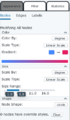
Figure 17. Node Appearance Menu
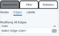
Figure 18. Edge Appearance Menu
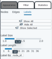
Figure 19. Label Appearance Menu


Network Algorithims

The last step of visualization using SNoMaN allows users to run some additional algorithms. As seen in Figure 20, these algorithms are divided into 3 subsections, Distance and Shortest Path, Efficient Distance Analysis, and Group-related functions.
The first subsection contains two buttons to run the average distance and shortest path algorithms which will add the calculated value to the variables for each node and change the bottom right graph to reflect this data.
The second subsection contains three alternative and newer metrics for distance analysis, local flattening ratio, k-fulfillment, and global flattening ratio. K-fulfillment and local flattening ratio are both metrics that describe local (dis)connection in the network, running either of these algorithms will also add their values to each node. Global flattening ratio is a single value for the entire dataset and represents a measure of the networks spatial tightness (Sarkar et. al, 2019).
Finally, the Group-related functions subsection allows the user to run the Louvain algorithm from Blondel et. al (2008) on the network to identify sub-communities within the node set. The algorithm also displays a number, known as the "Q-value" which represents the strength of the community partition, ranging from -1 to +1.
SSNtools - R Library
The initial intention of this tutorial was to provide an overview of Social Spatial Networking Tools in using the R programming language and the R packages "SSNtools", "tmap" and "igraph". However, the tutorial provided by the creators of the R package is very thorough, particularly in the area of the advanced statistical tools, if this is the type of analysis you would like to complete you can find that tutorial here. Due to this issue the focus on the tutorial changed to examining the visualization capabilities of the SNoMaN web app and the process of creating a SSN dataset. Future expansions to this tutorial may include an overview of the FriendlyCities tutorial that has been scaled down for a beginning audience.
References
Andris, C. (2019). Social Networks. The Geographic Information Science & Technology Body of Knowledge (2nd Quarter 2019 Edition), John P. Wilson (Ed.). DOI: 10.22224/gistbok/2019.2.9.
Andris, C., & Sarkar, D. (2022). Social networks in space. Chapters, 400-415.
Blondel, V.D., Guillaume, J.-L., Lambiotte, R. and Lefebvre, E (2008). Fast unfolding of communities in large networks. Journal of Statistical Mechanics: Theory and Experiment, 2008(10) P10008, 2008.
Bondy, J. A. (1982). Graph theory with applications.
Sarkar, D., Andris, C., Chapman, CA., & Sengupta, R. (2019) Metrics for characterizing network structure and node importance in Spatial Social Networks, International Journal of Geographical Information Science, 33:5, 1017-1039, DOI: 10.1080/13658816.2019.1567736
Tobler, Waldo R. 1970. “A Computer Movie Simulating Urban Growth in the Detroit Region.” Economic Geography (Supplement: Proceedings, International Geographical Union. Commission on Quantitative Methods), 46: 234–240. DOI:10.2307/143141.