User:KennethBatagon
Contents
- 1 Cycling in Carleton University: Calculating Fastest & Shortest Route and Determining Cycling Accidents
Cycling in Carleton University: Calculating Fastest & Shortest Route and Determining Cycling Accidents
Purpose
The purpose of this tutorial is to present the user with open-source data available using QGIS. Introduction. An open-source approach is a way of software product development and distribution in which the public is given free access to the source code. This enables users to access, change, and redistribute the programme in accordance with their requirements and preferences.
Introduction
The purpose of finding the shortest and fastest route between two points is to save time and reduce the cost of travel. This can be useful for individuals planning a trip and businesses or organizations that need to transport goods or people efficiently. For example, this tutorial calculates the shortest and fastest routes from an origin point, Carleton University, to the destination point, Walmart. For this tutorial, determining cycling collisions in the Carleton University and Walmart area helps to identify safe and efficient routes for cycling. This tutorial will use QGIS as it is a powerful and versatile GIS software that is widely used for mapping, spatial analysis, and data visualization.
Data Collection and Organization
QGIS
The first step for this tutorial is to get QGIS access. If you are using the school’s computer, you can skip this part.
QGIS Plugins
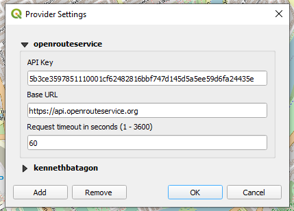
In order to calculate the fastest and shortest route, you will need to download a plugin within QGIS called ORS Tools (Open Route Service). The majority of the OpenStreetMap-based openrouteservice.org features are accessible through ORS Tools. Routing, isochrones, and matrix calculations are all part of the toolset and can be done interactively in the map canvas or via point files within the processing framework. Several attributes, including duration, length, and start/end locations, are set for output files. To do this, click Plugins -> Manage and Install Plugins and search for ORS Tools and install it. Once installed, proceed toward Web-> ORS Tools-> Provider Settings to request an API key. This is a crucial step as any parameters or actions you want to do will not work without the key. You will need to signup by searching open route service sign up or by clicking this link. Follow the instructions given in the email.
The second plugin is QuickMapServices. It serves as an accessible base map that perfectly complements the previous plugin, ORS Tools. As mentioned above, you will need to install this plugin through Plugins -> Manage and Install Plugins and search for QuickMapServices and install it. Follow the steps in Figure 3 and you should have a search menu on the right side of QGIS. Search up your preferred basemap. For this tutorial, I used RRZE OpenStreetMap Standard HD. After you clicked it, you should have the basemap under Layer on the left side of QGIS.
Open Data Ottawa
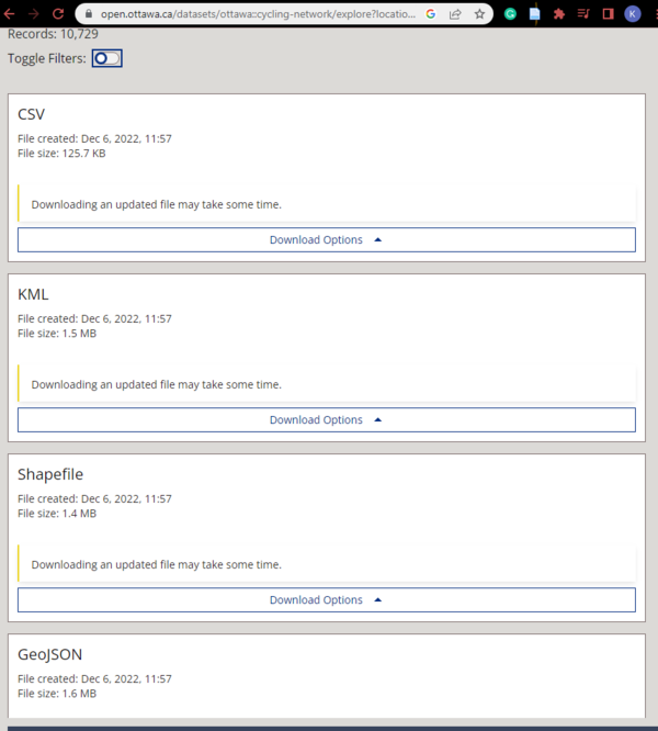
The next data collection can be found in Open Data Ottawa. The Open Data Ottawa platform is part of the City's open data initiative, which aims to make city data more transparent, accessible, and useful to the public. Hence, the shapefiles data we need is going to be extracted here. You will need a polygon shapefile for Ottawa Wards, traffic collision shapefile, cycling network shapefile, pedestrian network shapefile, and Ottawa roadlines shapefile.
Project Set up
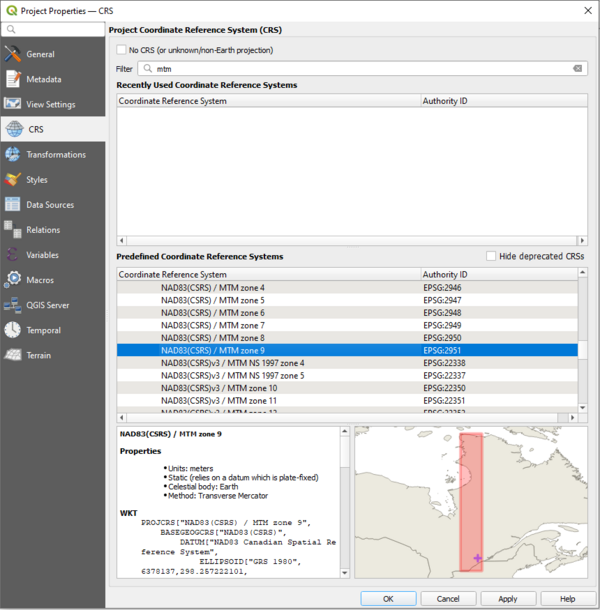
Before doing anything else, we need to set up the project coordinate system so it matches the data we collected from Ottawa shapefiles data. This can be done by clicking on Project-> Project Properties -> CRS and choose NAD83(CRS)/MTM Zone 9 as data of Ottawa suggested.
Calculating the routes using ORS Tools
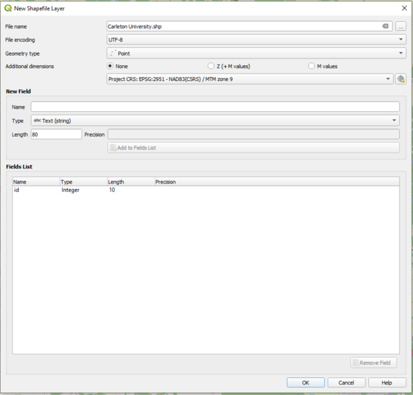
ORS Tools have three options for batch jobs. For this part of the tutorial, we will be working on the direction that calculates the fast and the shortest routes. First, you need to create a point layer as a shapefile (![]() ) as a setup for your origin and destination point.
) as a setup for your origin and destination point.
By doing so, it will pop up a point shapefile layer under the Layers category. Right-click on the newly created layer and click Toggle Editing. After that, Add Point Feature
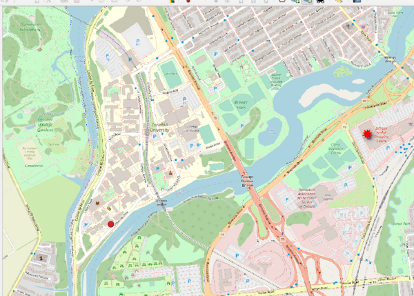
![]() should be available to click. Now begin adding a point feature for the origin point, Carleton University, and find Walmart in Billings Bridge as the destination point as shown in Figure 7. I added my origin layer to Loeb Building as it is our department building.
should be available to click. Now begin adding a point feature for the origin point, Carleton University, and find Walmart in Billings Bridge as the destination point as shown in Figure 7. I added my origin layer to Loeb Building as it is our department building.
Fastest Route
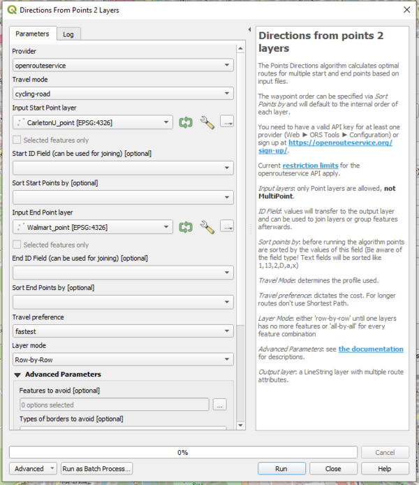
After creating the point layers, it is time to open up ORS Tools. Web-> ORS Tools-> Batch Jobs->Points (2 Layer). It should give you an image similar to Figure 6. First, we start with the fastest route. Set Carleton as the Input Start Layer and Walmart as the end point layer. Set Travel Mode to cycling-road and Travel preference to fastest and run it.
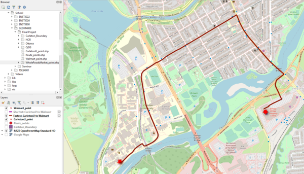
By doing so, you should get the fastest route from Carleton University to Walmart.
Shortest Route
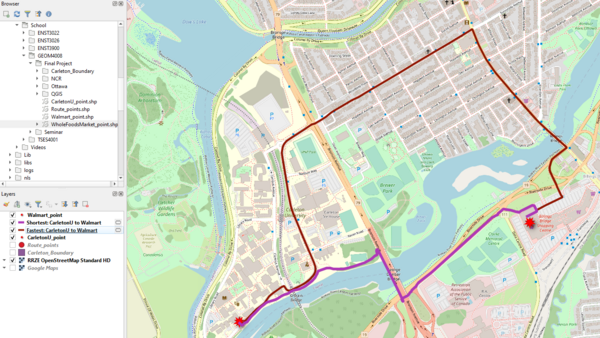
For the shortest route, do the same steps as mentioned above. However, change the Travel preference to shortest. You should get the following image:
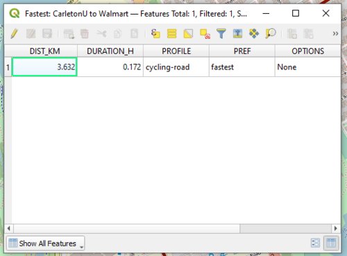
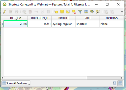
This indicates that the shortest route does not always mean the fastest due to multiple factors such as traffic, traffic lights, and bike routes. This is proven by opening the attributes table for both the fastest and shortest route layers under Layers category. You can get access to the attribute table by right-clicking the fastest and the shortest route and click Open Attribute Table.
Isochrones
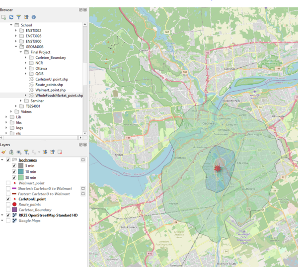
In this plugin, we can also estimate the distance where one can cycle around the campus in a given time. In this case, we are putting 5 minutes, 10 minutes, and 30 minutes distance around the campus. It gives a fairly accurate estimate if an individual wants to explore the capital ward through cycling. Open ORS Tools again and select Isochrones form Point -> Travel mode as cycling-regular, pinpoint Carleton University for the Input Point from map canvas, select Dimension as time and put 5,10,30 for the Comma-separated ranges [min or m], and run it. As seen in Figure 12, 30 minutes of travel time can potentially cross the border of Quebec by just cycling from the campus. If one wants, the isochrone function can be another way around. It could be based on how far can one cycle from campus using displacement as a range.
Analyzing Cycling Accidents around the Campus Area
Adding the Data
For this part of the tutorial, we need to add the shapefiles we downloaded from Open Data Ottawa. You can do this by going to the Layer -> Add Layer -> Add Vector Layer. The vector dataset should be from your working directory or where you saved the downloaded shapefiles.
Attribute Table
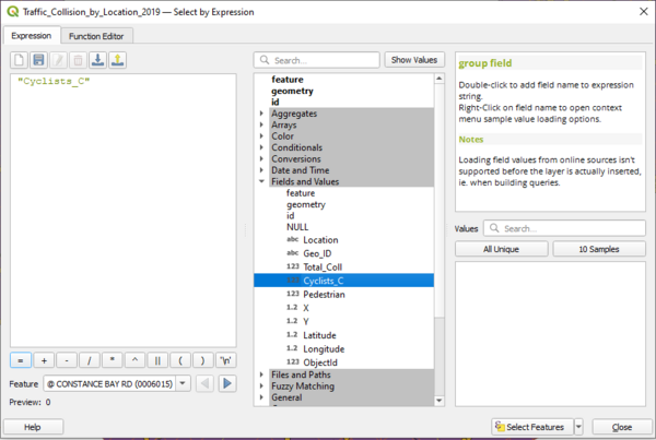
After that, we need to edit the attribute table of the traffic collision shapefiles as it includes several transportation methods and this part's objective is to determine mainly cycling collisions. We can do this by right-clicking the traffic collisions and opening the Attribute Table. We can edit the table by Select features using an expression![]() . Open up the Field and Values and choose Cyclist_C.
. Open up the Field and Values and choose Cyclist_C.
After you selected the feature, various points should be highlighted and we need those to be their own separate data layer. We can do that by exporting the selected feature as a new layer. Right click Traffic collisions -> Export -> Save Selected Features as shown in Figure 14. A new layer should popped up and you need to save that layer permanently.
Setting Boundaries
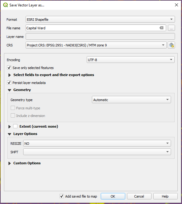
Since the goal of this tutorial is around the campus, we need to trim the Ottawa Ward where Carleton University is located. According to the City of Ottawa, Carleton University is located within the capital ward, ward 17. Thus, clipping is necessary to isolate this ward. Right-click on Wards_2022-2026 -> Open Attribute Table -> Select features using an expression. In the Attribute Table, open Field and Values and select WARD so it can be put in the expression and choose = and 17 under the unique values. The = sign shows that the values of the two expressions are equal to each other. The location of Ward 17 or Capital Ward should be highlighted on your project. Similar to the previous instructions, clip the capital ward into a new featured layer as this is the main area we are going to work with. You need to make sure that the projected coordinate system is the same to the one we set up earlier.
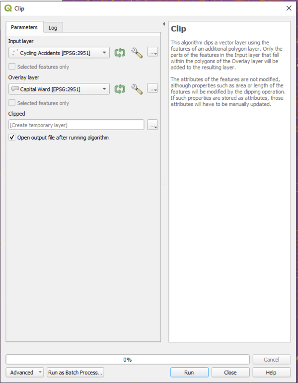
Now that the base of operation is clipped, we need to clip all the other data along with it so points and polygons does not overlap from the capital ward. This can be done by going to the Vector on the menu -> Geoprocessing Tools -> Clip. In the Parameters the Input Layer will always be the data that goes within the Overlay Layer, which is the Capital Ward. Repeat this step for all the data needed.
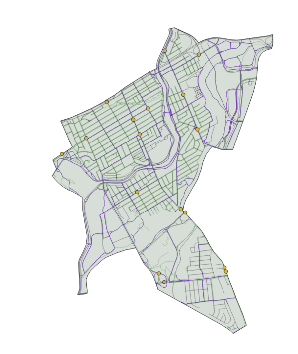
After clipping all the necessary data within the capital ward, the result should be somewhat like Figure 17.
Conclusion
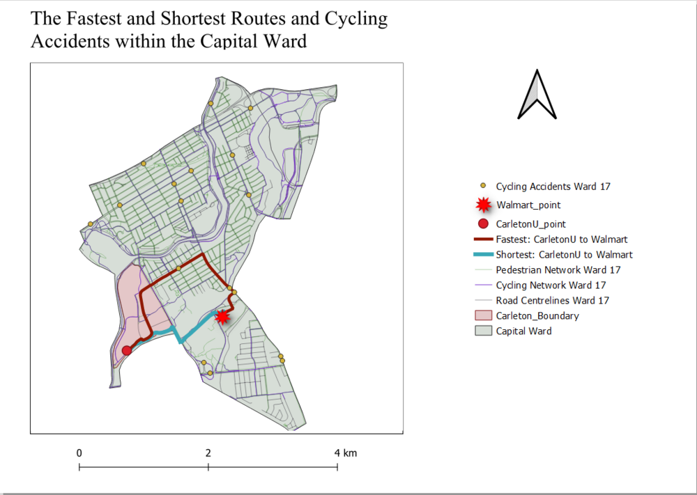
In this tutorial, we found out that the shortest route does not always mean the fastest due to multiple factors such as traffic, traffic lights, and bike routes. The fastest route has a distance of 3.62 km and it takes around 10 minutes and 30 seconds to reach the final destination. On the other hand, the shortest route has a distance of 2.15 km but it takes 14 minutes and 46 seconds to reach the destination. We learned that 30 minutes of cycling can take an individual to cycle around Ottawa's downtown area and even Gatineau, Quebec. Additionally, 5 minutes of cycling does not take one to travel to a much greater area. In the final map showing the routes and cycling accidents, taking the fastest route from campus to Walmart seems to be dangerous due to multiple cycling accidents. The shorter route tends to be the best option in terms of safety as there is only a 5-minute difference between the two routes.
References
- Canadian Open Data and Free Geospatial Data. (2010, October 26). https://canadiangis.com/data.php
- Clerk, O. of the C. (2022, December 14). Ottawa Ward Boundary Review 2020. https://ottawa.ca/en/city-hall/public-engagement/projects/ottawa-ward-boundary-review-2020
- Open Ottawa. (2022). https://open.ottawa.ca/
- Service Area Analysis using Openrouteservice (QGIS3)—QGIS Tutorials and Tips. (n.d.). Retrieved December 22, 2022, from https://www.qgistutorials.com/en/docs/3/service_area_analysis.html

