Using FUTURES in GRASS for Modelling Urban Growth
Using FUTURES in GRASS for Modelling Urban Growth
Contents
Introduction
The aim of this tutorial is to demonstrate the use of FUTURES (Future Urban-Regional Environment Simulation) for urban spatial growth analysis. While most urban growth models are focused on cell-level conversions and object-based representation, FUTURES uses patch-based, stochastic, multi-level land change modelling framework to provide urban-rural land development models. FUTURES is an open source urban growth model that is designed to address regional-scale ecological and environmental impacts of urbanization and captures the spatial structure of development. This is done through regional projections of landscape patterns and then FUTURES creates submodels that integrate nonstationary drivers of land change. In this tutorial, the submodel that will be used is site suitability (POTENTIAL submodel). The POTENTIAL submodel uses a set of coefficients that relate a selection of site suitability factors to the probability of a place becoming developed. The model does this through multilevel logistic regression through a hierarchy of characteristics based on land use systems and the divergent relationships between predictor and response variables to obtain the coefficients.
Part 1: Getting Started
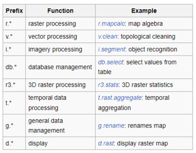
In order to complete this tutorial, basic GRASS functionality is required . GRASS GIS provides standard GIS tools and graphical user interface for model uses and for FUTURE modelling, GRASS GIS simplifies the distribution of FUTURES by providing efficient libraries for GRASS GIS. FUTURES in GRASS GIS has multiple advantages for model users including its multiplatform, its scriptability (Bash, Python, R), graphical user interface and can be used for further analysis as well as visualization. GRASS has a variety of different modules that can be used to prepare and analyze data layers. It is important to note that commands have a specific syntax in order to produce the results that are desired.
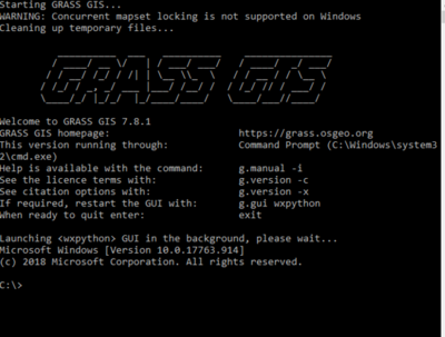
Launching the Graphical User Interface (GUI) in the mapset. The GUI can be found in the top menu bar labelled layer manager and it allows for the display as well as manipulating the raster and vector data. GRASS modules can be executed on either GUI or command line interface. Through this tutorial commands lines can be copied into the GUI command console or in the command window and pressing enter after each command.
Software
Software requirements to run FUTURES in grass can involve many types of software depending on the model that is required. For this tutorial, the software needed is GRASS GIS 7, the submodel addon (r.futures.potential) and R Software. Easily install package:
g.extension r.futures
g.extension r.sample.category
R packages can be installed using the command line terminal which was started with GRASS GIS and R. :
R
Data
This tutorial will mainly using FUTURES with Future Transit and LRT stations in Ottawa and Ottawa's Business Improvement Areas (BIA) using the R command line. Using these two datasets, the main objective is computing the distance between the two data sets. Looking at gaps in the development, allows for identification of areas for site suitability for more connectivity in these systems through urban growth. The Potential Submodel requires raster maps that are predictors that drive land change. This can include counties, slope, road density, forests, and/or distance to protected areas etc. which is used as existing data on urban regional land cover.
Part 2: Modelling
Firstly, the study extent and resolution can be specified with the command below. This command manages the boundary definitions for the geographic region. In GRASS the region refers to a geogrpahic area that has defined boundaries based on the map projection.
g.region
For this tutorial we will use distance to roads in km and development pressures. The POTENTIAL model requires a set of uncorelated predictors that drive land change. This will create predictors needed for the POTENTIAL submodel.
r.grow.distance input=roads distance=roads_dist
r.mapcalc "roads_dist_km = roads_dist/1000."
This generates a raster map containing distances to nearest raster features and/or the value of the nearest non-null cell.
r.grow.distance input=transit_station distance=dist_to_transit_system
This can be modelled using r.futures.potential POTENTIAL also requires subregions data. To compute the subregions of this tutorial, the counties data is made into raster data
v.to.rast input=counties type=area use=attr attribute_column=FIPS output=counties
The predictors and their coeffiecient can be placed into a csv file. the command for this is as follows:
predictors-slop.dist_to_transit_system_params=potential.csv
POTENTIAL submodel uses a combination of the site suitability factors through mapped predictors. To compute POTENTIAL model:
r.futures.potential input=sampling output=potential.csv columns=devpressure_0_5_92,road_dens_perc,forest_1992_smooth_perc,dist_to_water_km,dist_to_protected_km developed_column=urban_change_clip subregions_column=counties --o
Conclusion
This tutorial is an introduction of how GRASS can be used to model land development by displaying the connection of the new Ottawa transit system to the proximity of commercial areas in the city of Ottawa. FUTURES is a tool that is able to create a variety of land development models and the site suitability , POTENTIAL submodel, is showcased in this tutorial.
References
Meentemeyer, R. K. (2018, September 14). GRASS GIS Manual: r.futures. r.futures grass gis manual . Retrieved December 23, 2021, from https://grass.osgeo.org/grass78/manuals/addons/r.futures.html

