Watershed Analysis to determine the ancient/contemporary pathways of water flows to understand trend of floods
Contents
Introduction
The integrated management of floods on the scale of the watershed area offers interesting prospects for making a relevant diagnosis and finding solutions for managing the hazard, particularly upstream of the stakes. Therefore, the present paper sheds light on the watershed analysis in order to identify the water flows as well as catchments that will allow an understanding of the trend of floods over time. The said flood management is nowadays feasible thanks to GIS or SDSS as effective means that helps decision-makers improve their results and obtain a notable gain in terms of time and accuracy. So, the QGIS software is considered an SDSS able to ingest spatial and non-spatial data in order to perform mapping and spatial analysis with the aim of providing decision-makers with concerts outputs that will help in understating the flood trends and hence increase the rapidity of intervention in case of hazards or naturals risks related to floods. The watersheds analysis will rely on hydrological modeling of the basin of Haiti using a Digital Elevation Model (DEM) of 30 m resolution (cell size) in order to determine the hydrological network or flow waters and so to understand how floods behave over time knowing the pathways of streams.
Purpose
The purpose of the current document is to conduct a watershed analysis using DEM data and QGIS software for water flows and catchment identification in order to understand flood variation over time by comparing the pathways over time. Subsequently, the study uses elevation data from which several products will be derived such as slope, aspect, and shaded relief, and also flow waters and catchments will be extracted. Subsequently, the study will compare the water flow pathways using two DEM spaced at least 8 years apart. The study will as well target some aspects of spatial analysis, spatial interpolation, and 3D modeling using QGIS software and some plugins installed on it.
Region Of Interest (ROI)
The analysis will take as Region Of Interest (ROI) the Môle-Saint-Nicolas arrondissement in the Nord-Ouest Department of Haiti as shown in the following map:
.jpg)
Figure 1. Region Of Interest (ROI)
Software
The software used is QGIS version 3.24.2 for Windows OS. It’s a free and open-source GIS tool directly downloadable via the link Download QGIS. We will use also the 3D Builder tool to visualize 3D objects in STL format that we will obtain from our DEM using the DEMto3D plugin installed on QGIS. The tool can be freely downloaded via How to use 3D Builder for Windows - Microsoft Support

Figure 2.3d builder software

Figure 3. QGIS software
Some QGIS plugins are installed in order to benefit from more functionalities and options, such as: • QuickMapServices: plugin to add base maps like Goole, OSM, Bing…
• DEMto3D: a plugin that allows 3D printing of terrain models (DEM).
• Qgis2threejs: plugin for 3D visualisation on web browsers.
Data
Spatial data types
There are two main types of geographic data in GIS: 1. Matrix: more often called "Raster", correspond to grids composed of cells (like an "image" composed of pixels). Each cell contains a value that often represents a geographical phenomenon, for example, altitude or land use. It can be a scanned map, an aerial photograph, a satellite image, a digital photo, a DTM (Digital Terrain Model)... 2. Vector: they are composed of points, lines or polygons. The most common vector file format in GIS is the "shapefile" format.
Used data
All the data used for this study is free and available for download, they are summarised in the following table:

Table 1: Data
Tutorial
DEM acquisition
The analysis of watersheds is based on the delineation of catchment areas that can be done using a Digital Elevation Model (DEM) and the derivation of different relief features. Before starting the actual analysis, we will need to obtain elevation information about the study area in the form of a DEM (a raster with cell values corresponding to the elevation). Thus, the quality of the hydrological analysis in general, and the accuracy of the delineation of a catchment area, in particular, will depend on the quality of the DEM (spatial resolution, presence of bad pixels, etc.). For the purpose of this study, we have downloaded the two DEMs from Download|ASTER GDEM and from ASF Data Search (alaska.edu). The ASTER GDEM provides users with the third version (released on August 5, 2019) of the Advanced Spaceborne Thermal Emission and Reflection Radiometer (ASTER) Global Digital Elevation Model (GDEM). The said version maintains the GeoTIFF format and the same gridding and tile structure as in previous versions, with 30-meter spatial resolution and 1°x1° tiles, and adds additional stereo-pairs, improving coverage and reducing the occurrence of artifacts. The refined production algorithm provides improved spatial resolution, and increased horizontal and vertical accuracy that was calculated by comparison with more than 23,000 independent reference geodetic ground control points from the U.S. National Geodetic Survey. The root means square error (RMSE) measured for GDEM v3 is 8.52 meters. While the ALOS PULSAR DEM belongs to the creation of radiometric terrain corrected (RTC) products as a project of the Alaska Satellite Facility that makes SAR data accessible to a broader community of users. The project corrects synthetic aperture radar (SAR) geometry and radiometry and presents the data in the GIS-friendly GeoTIFF format. In this context, we have downloaded two tiles to cover the ROI for each DEM as shown in the map below:

Figure 4: DEM tiles
As pointed out above, several DTM files (several tiles or several images) may be needed to cover the area of interest. In this case, a mosaic ("merge") of the different files will be needed to obtain one single file using the “Merge” function of QGIS.

Figure 5. Merge function
Coordinate Reference System
The Coordinate Reference System is an important element in our project that we should check with high prudence since it could easily affect our spatial analysis and further geo-processing operations. In particular, we should ensure that you use the correct coordinate system for our project (for this exercise on Haiti, the CRS used is: "WGS 84 UTM Zone 18N, EPSG: 32618"). Therefore, we will re-project the DEM raster from WGS84 (EPSG: 4326) to WGS 84 UTM Zone 18N, EPSG: 32618" using “Wrap” function used for raster re-projection:

Figure 6. Wrap function for re-projection
While we use Wrap for raster data type, we use “re-project layer” for vector data type as follows:
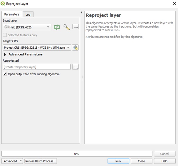

Figure 7. Re-project layer for vector data
Clipping the DEM based on the ROI
When working on grid layers, it’s preferable to focus on the ROI instead of processing the whole data. Thus, we will perform a spatial clipping (optional) of the DEM to reduce its spatial extent which can be useful to reduce the file size and hence speed up the execution of the following tools. The function used is “Clip Raster by Mask Layer”:

Figure 8. Clip Raster by Mask Layer
Here is below the DEM merged, clipped and re-projected:

Figure 9.DEM merged, clipped and re-projected
DEM correction
A Digital Elevation Model is a representation of the elevations of a territory. Each cell (pixel) of this DEM contains a height value. Depending on the means of generating this surface and the size defined for the cells, the height assigned to the cell is more or less close to the exact reality. So, if we want to use the DEM for a 3D view of the territory (with Qgis2threejs, for example), we can use it as is and without any particular precaution. However, if we want to model the flow of water on the surface of this territory, the first and most important thing to do is to correct and adapt it to this objective. The quality of the results obtained with regard to the catchment areas and the various possible hydrological calculations depends on what we do in this step. A common correction is to look for cells surrounded by higher cells. These troughs will cause a problem when determining the flow directions, as the algorithm cannot leave the trough. In the DTM pre-processing, these troughs are filled in until an adjacent cell is found that is lower than the filling height. This cell will then be the outlet cell for the flow calculation.
The sinks fill can be performed through different functions in QGIS such as:
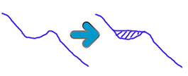

Figure 11. DEM sinks fill
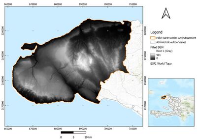

Figure 12. DEM filled
Deriving products from DEM
The DEM is a rich data source from which we can derive a multitude of products such as slope, aspect and shaded relief. • Slope

Figure 13. Slope function in degrees

Figure 14. Slope from DEM
• Aspect

Figure 15. Aspect calculation

Figure 16.Aspect from DEM
• Hillshade ( shaded relief)

The aspect map identifies the compass direction that the downhill slope faces for each location. • Hillshade ( shaded relief)
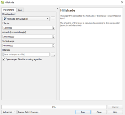
Figure 17. Hillshade function
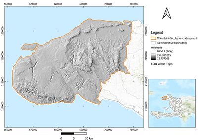

Figure 18: Hillshade from DEM Hillshade function creates a 3D grayscale representation of the terrain surface, taking into account the relative position of the sun to shade the image. Shading is a technique for visualizing terrain determined by a light source and the slope and appearance of the elevation surface. It is a qualitative method for visualizing the topography and does not give absolute elevation values.
3D visualisation
3D visualisation allows an improved quality of terrain reality thanks to DEM data, and hence we can drape a satellite image (Google for example) on the DEM for the same area. Let’s see how it looks for our case of study: The plugin used is Qgis2threejs and the data ingested by it is the DEM as well as Google satellite imagery.

Figure 19.3D visualization of the DEM with Google imagery
We can also export our DEM (Tiff format) as a 3D object in STL format, for that we can use the DEMto3D plugin.
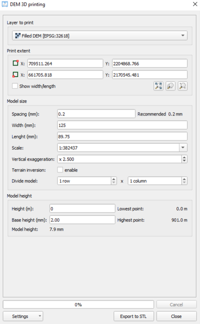

Figure 20. DEMto3D plugin
The output is 3D object is STL format, that we will open via 3D Builder tool:

Figure 21: DEM exported as STL file
Watersheds analysis
The watersheds analysis will be based on streams extraction from our DEM. Hence, there are several options to perform this process using QGIS software: Channel Network and Drainage Basin; R.Stream.Extract.
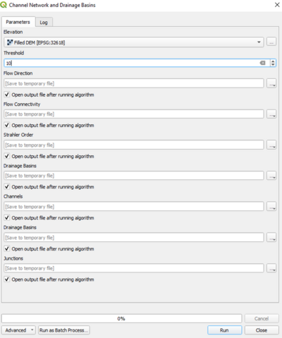

Figure 22. Channel Network and Drainage Basins

Figure 23. r.stream.extract
The parameter “Minimum flow accumulation for streams” defined as a threshold determines the minimum (optionally modified) flow accumulation value that will initiate a new stream. Among the outputs of these geoprocessing tools, we have streams and flow direction layers. The former establishes to which cell the water flows, starting from the central cell. To do this, it calculates the slope between the central cell and the 8 surrounding cells. He assumes that the water flows to the cell with the steepest slope.

Figure 24. Flow direction example In this example, the steepest slope is 128, hence the water flows from the central cell to the cell with 128 as the value.
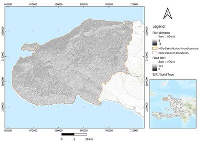

Figure 25. Flow direction The water flow pathways generated from ASTER GDEM DEM which is referring to the contemporary context are given by the next map:
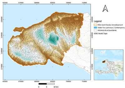

Figure 26. Contemporary water flow pathways The above map shows the generated stream network from the ASTER GDEM DEM. Regarding the ancient water flow pathways, we will use the ancient DEM that’s from ALOS PULSAR in order to extract streams. The map below shows the spatial distribution of the water flow pathways
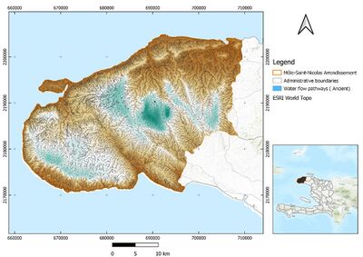

Figure 27. Ancient water flow pathways
From the two maps, we can figure out the water pathways variations over time. Furthermore, we will overlay the layer of flood zones on both of them to have a more concrete visualisation of the flood trends throughput water flow pathways evolution over time.

Figure 28. Contemporary water flow pathways with flood zones The water flow pathways differ in the two maps which refer to different dates and reflect the spatial-temporal variation over time. Furthermore, the overlaid flood zones layer allows more identification of the said variation since it points out the differences in pathways in the flood zones.

Figure 29. Ancient water flow pathways with flood zones
Conclusion
Throughout this study, we have demonstrated how to conduct a watersheds analysis using DEM data in order to determine the water flow pathways variations for flood trend identification. The study case was carried out using QGIS software and some plugins. Moreover, the current project can be extended by working on several DEM issued on different dates so that we have a multi-temporal spatial assessment of the water flow pathways. Such analysis would help decision makers improve their comprehension of the risks as well as taking accurate decisions in a rapid time frame, and that’s thanks to GIS/SDSS evolution.
References
ALOS PALSAR - Radiometric Terrain Correction | ASF (alaska.edu)
New Version of the ASTER GDEM | Earthdata (nasa.gov)
Hydrologie | Blog SIG & Territoires (sigterritoires.fr)
Spatial decision support systems: An overview of technology and a test of efficacy M.D. Crossland ,B.E. Wynne , W.C. Perkins
Initiation à ArcGIS - Travaux pratiques sur les Systèmes d'Information Géographique – SIG Denis, Antoine 2012