Difference between revisions of "Landscape Change Assessment using Unsupervised Image Classification in GRASS GIS"
| Line 3: | Line 3: | ||
==Introduction to GRASS GIS== |
==Introduction to GRASS GIS== |
||
| − | [[File:LT_GrassLogo.png| |
+ | [[File:LT_GrassLogo.png|thumb|100px|GRASS GIS Logo]] |
Revision as of 21:27, 15 December 2019
Contents
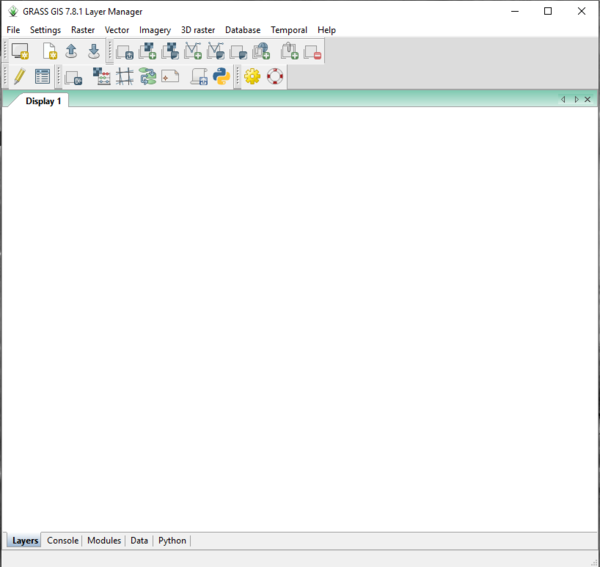
- 1 Purpose
- 2 Introduction to GRASS GIS
- 3 Methods
- 3.1 Software Download and Installation
- 3.2 Data Set
- 3.3 Starting GRASS GIS
- 3.4 Adding Extensions
- 3.5 Importing Landsat Rasters
- 3.6 Visualizing Layers
- 3.7 Raster Smoothing and Discontinuity Maps
- 3.8 Image Grouping
- 3.9 Pre-Processing
- 3.10 Unsupervised Classification
- 3.11 Landscape Change Assessment
- 3.12 Editing the Landscape Change Maps for Distribution
- 3.13 Not Covered in this Tutorial
- 3.14 Additional Resources
- 4 Conclusion
- 5 References
Purpose
The purpose of this tutorial is:
Introduction to GRASS GIS
Methods
Software Download and Installation
In this tutorial, GRASS GIS version 7.8.1 for Windows is being used, however this software is also available for Mac and Linux users. The latest version of GRASS GIS may be downloaded here. This website contains very useful information and documentation for users that have never been exposed to GRASS GIS before now. I highly suggest looking at this documentation, as well as this tutorial which provides more information on GRASS GIS.
Data Set
Because this tutorial is being written to demonstrate the ability of GRASS GIS to assess changes in landscapes, a data set has been provided for the user. There are many sources where one can find satellite imagery data, however a data set is being provided to the user so they may follow along with this tutorial without having their own data set. This data set consists of two GeoTiff files acquired using the Earth Observing System (EOS) Landviewer tool. These GeoTiff files contains an image obtained by Landsat 7 on September 7, 2000 and an image obtained by Landsat 8 on September 23, 2017. Both images contain imagery of the same area of interest (AOI) which consists of a 40.04 km² square area centered at 45.03001°N 75.68135°W. This area is located in Kemptville, Ontario, an area which has undergone development since the early 2000s to accommodate for increased population sizes. The population of Kemptville is expected to rise given it's close proximity to Ottawa, making it an ideal location for commuters to reside, which means that further development is also expected.
| Landscape Change Assessment Data Set | |
|---|---|
| Data Information | Data File |
| GeoTIFF file for raster imagery from September 7, 2000 with bands 2, 3, and 4 (Landsat 7) | September 2000 File |
| GeoTIFF file for raster imagery from September 23, 2017 with bands 2, 3, and 4 (Landsat 8) | September 2017 File |
| GeoTIFF file for raster imagery from September 7, 2000 with bands 1, 2, and 3 (Landsat 7) | [September 2000 Visible Bands File] |
| GeoTIFF file for raster imagery from September 23, 2017 with bands 1, 2, and 3 (Landsat 8) | [September 2017 Visible Bands File] |
Starting GRASS GIS
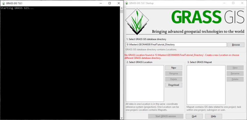
Once GRASS GIS is properly installed on your computer, you may locate it and open the program.
Figure 1: Screenshot of GRASS GIS Startup Interface
- 1)
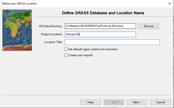
Figure 2: The Define New GRASS Location window where the user selects a data directory and project location.
- 1)
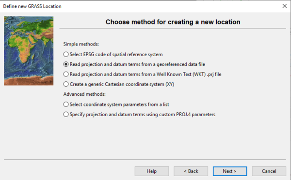
Figure 3: The Define New GRASS Location window where the user chooses a method for creating a new location.
- 1)
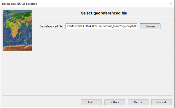
Figure 4: The Define New GRASS Location window where the user selects a georeferenced file.
- 1)
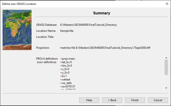
Figure 5: The Define New GRASS Location window summary page.
- 1)
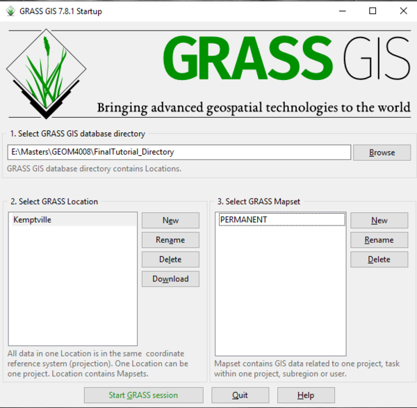
Figure 6: The GRASS Startup window with a Directory, Location, and Mapset selected.
- 1)
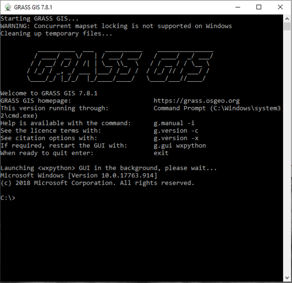
Figure 7: The GRASS Command window.
- 1)
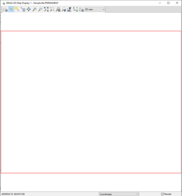
Figure 8: The GRASS Map Display window.
- 1)
Figure 9: The GRASS Layer Manager window.
Adding Extensions
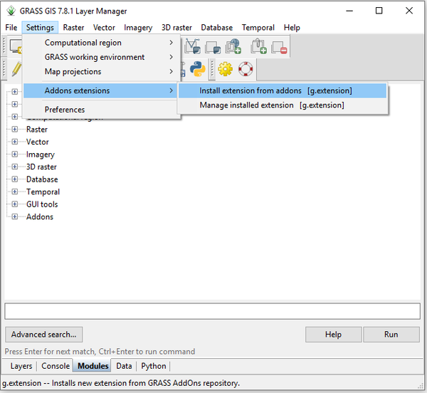
Figure 10: The path to install new add-ons in GRASS GIS.
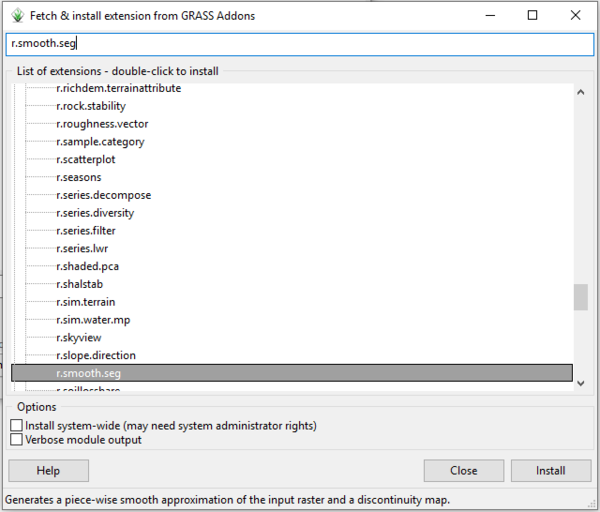
Figure 11: The "Fetch & Install Extension from GRASS Add-ons" window with search results for the r.smooth.seg add-on.
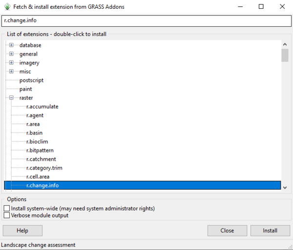
Figure 12: The "Fetch & Install Extension from GRASS Add-ons" window with search results for the r.change.info add-on.
- 1) At this point, GRASS GIS must be closed and restarted. Upon opening GRASS GIS for the second time, navigate to the Modules tab at the bottom of the Layer Manager window.
- 2) Click the + sign beside the Addons category to expand it.
- 3) Double-click on the add-on to run the selected module, or select it and press "Run" in the bottom right corner.
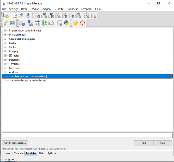
Figure 13: The Layer Manager window with the Modules tab open, and the newly installed add-on selected.
Importing Landsat Rasters
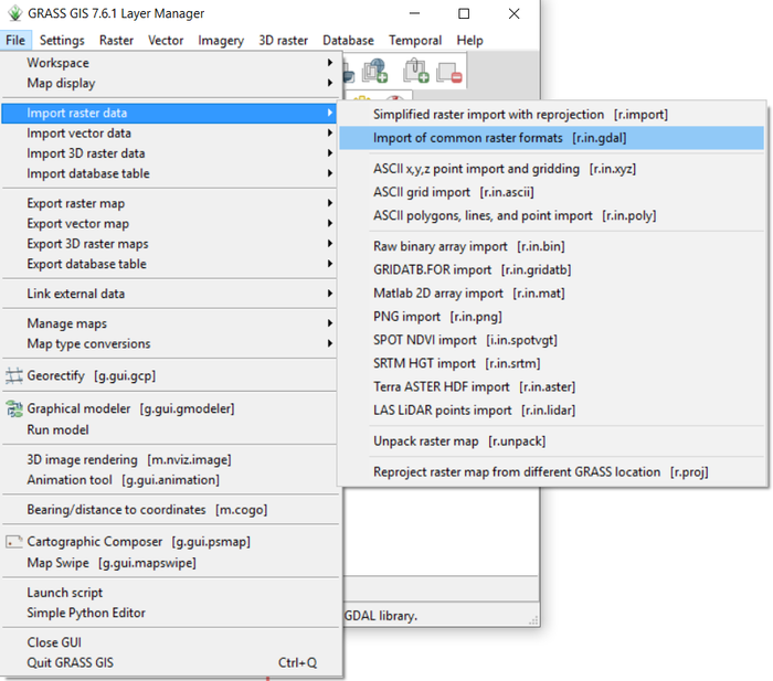
r.in.gdal [(https://grass.osgeo.org/grass78/manuals/r.in.gdal.html]
- 1)
Figure 14: The path to import raster data using the r.in.gdal module.
- 1)
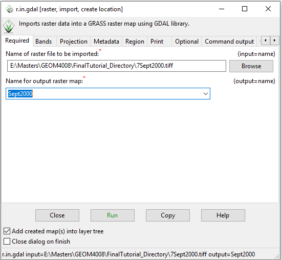
Figure 15: The r.in.gdal module window showing input and output raster information on the Required tab.
- 1)
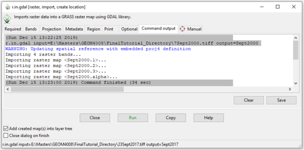
Figure 16: The r.in.gdal module window showing the Command Output tab.
- 1)
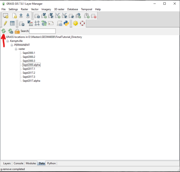
Figure 17: The "Refresh" button on the Data tab in the Layer Manager window.
Visualizing Layers
- 1)
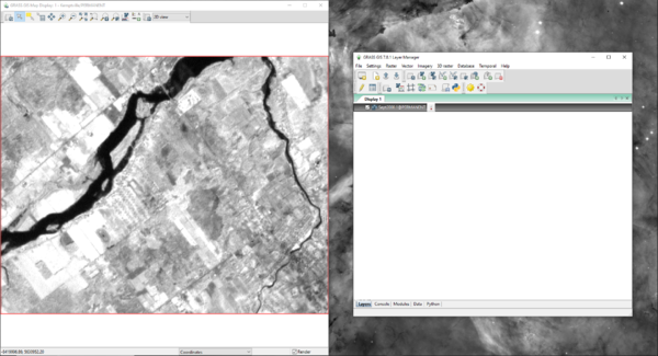
Figure 18: The Map Display window and Layer Manager window showing the Sept2000.1 layer.
d.rgb [1]
- 1)
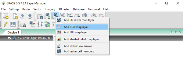
Figure 19: The path to add an RGB map layer using the d.rgb module.
- 1)
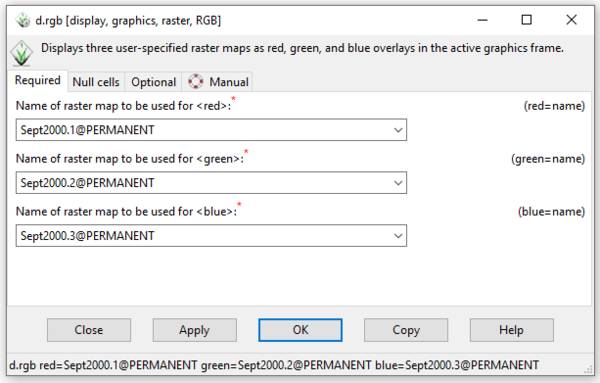
Figure 20: The d.rbg module window showing the required input raster information.
- 1)
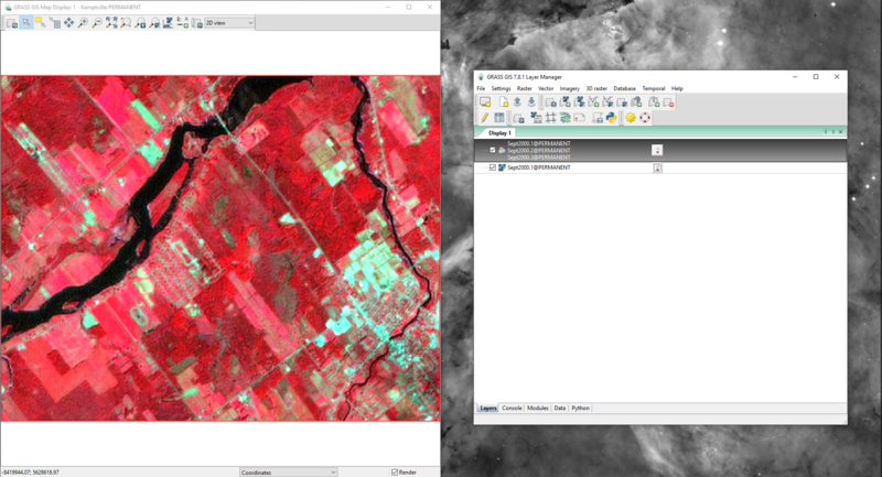
Figure 21: The RGB map layer output in the Map Display window and the selected RGB map layer in the Layer Manager window.
- 1)
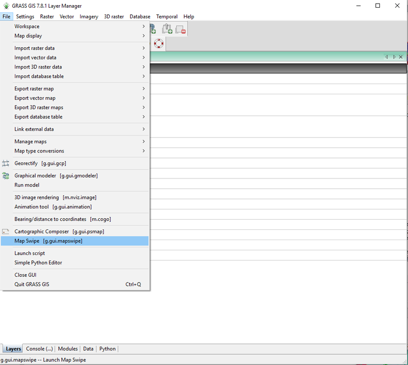 Figure 22: The path to use GRASS Map Swipe with the g.gui.mapswipe module.
- 1)
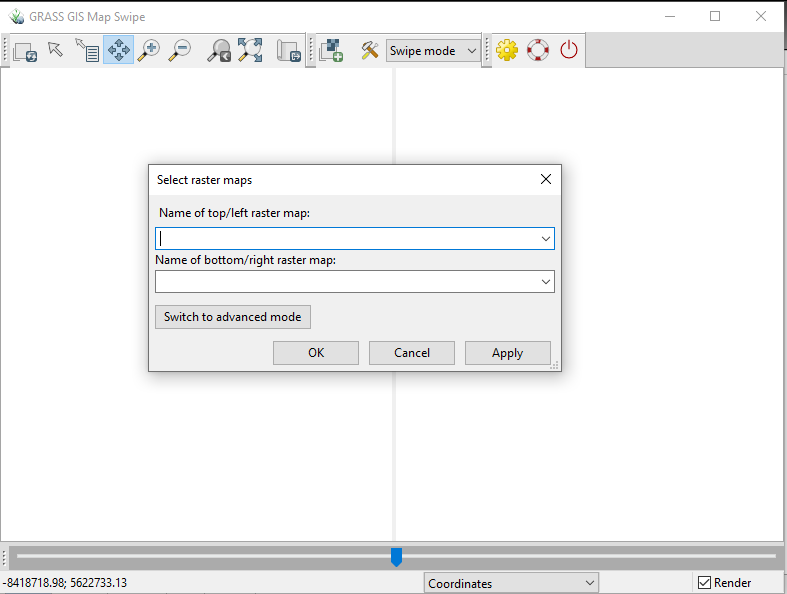 Figure 23: The Select Raster Maps window from the Map Swipe module.
- 1)
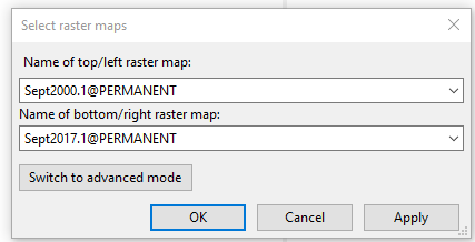 Figure 24: The completed Select Raster Maps window.
- 1)
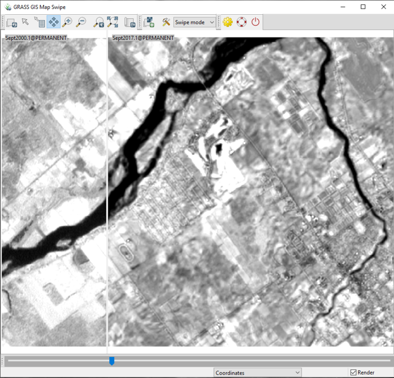 Figure 25: The Map Swipe window with displaying band 1 of the September 2000 image on the left, and band 1 of the September 2017 image on the right.
- 1)
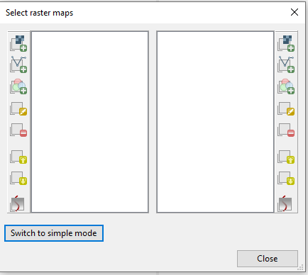 Figure 26: Advanced mode of the Select Raster Maps window showing many different options for selecting layers to compare using the g.gui.mapswipe module.
Raster Smoothing and Discontinuity Maps
r.smooth.seg - image pre-processing (takes place before segmentation - smooths out each band individually - also identify segments from each individual band)
- 1)
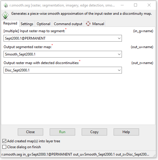 Figure 27: The r.smooth.seg module window with the completed input and output information on the Required tab.
- 1)
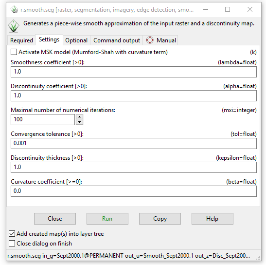 Figure 28: The Settings tab in the r.smooth.seg module window showing the different variables that can be adjusted.
- 1)
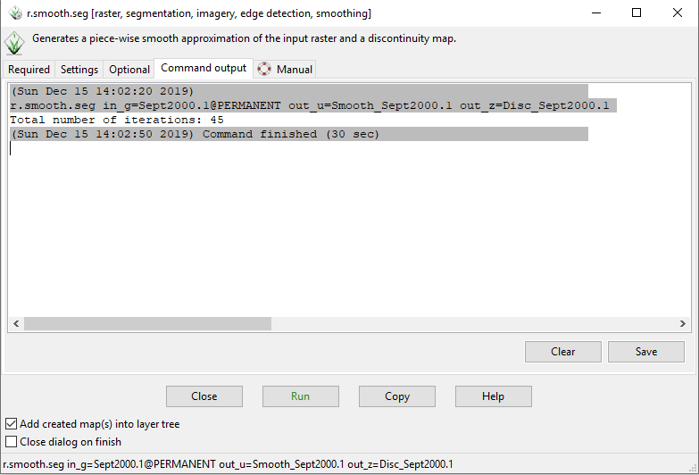 Figure 29: The Command Output tab in the r.smooth.seg module window showing the output information.
- 1)
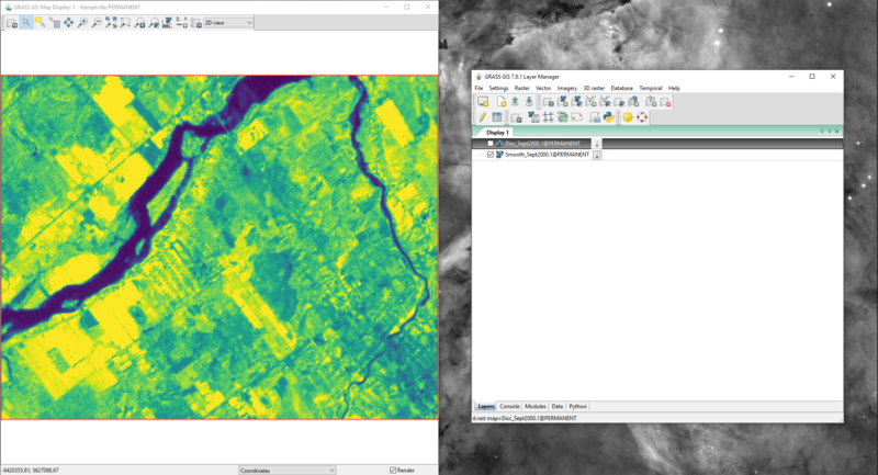 Figure 30: The Map Display for the smoothed map output for band 1 of the September 2000 data using the r.smooth.module module.
- 1)
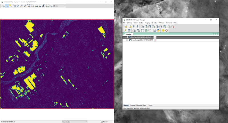 Figure 31: The Map Display for the discontinuity map output for band 1 of the September 2000 data using the r.smooth.module module.
Image Grouping
i.group - group bands 2, 3, 4 together, and create a subgroup containing all 3 of the images (sub-groups required for the cluster step - group and subgroup contain the same (all 3) images)
- 1)
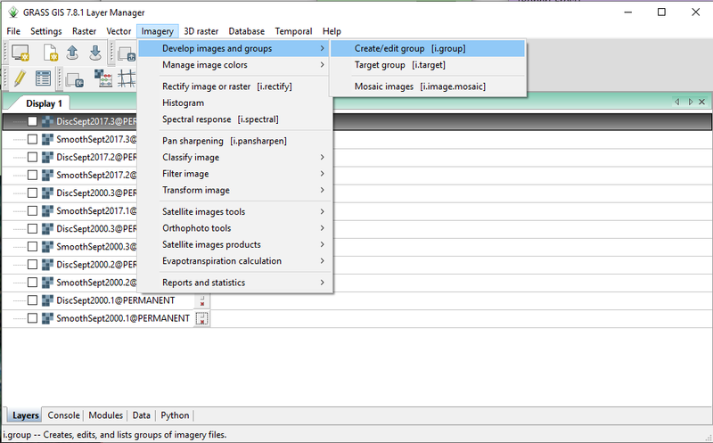 Figure 32: The path to the i.group module in the Layer Manager window.
- 1)
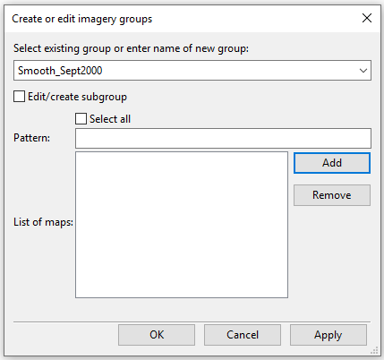 Figure 33: The Create Imagery Groups window from the i.group module.
- 1)
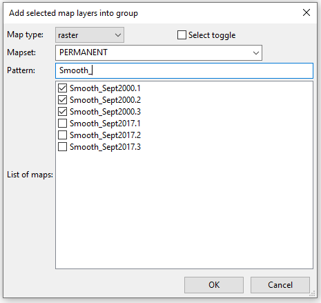 Figure 34: The Add Selected Layers into Group window from the i.group module.
- 1)
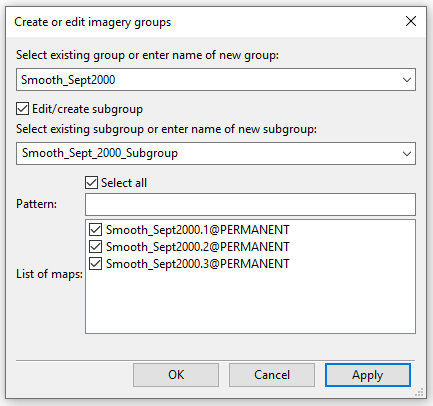 Figure 35: The Create Imagery Groups window showing the creation of a subgroup using the i.group module.
Pre-Processing
i.cluster (Generates spectral signatures for land cover types in an image (the subgroup containing all 3 bands we used above) using a clustering algorithm - this is creates the input for the maxlik tool)
- 1)
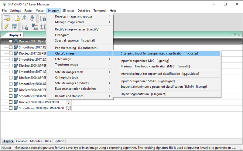 Figure 36: The path to the i.cluster module in the Layer Manager window.
- 1)
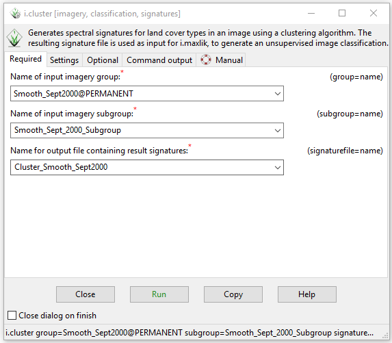 Figure 37: The i.cluster module window showing the input and output information on the Required tab
- 1)
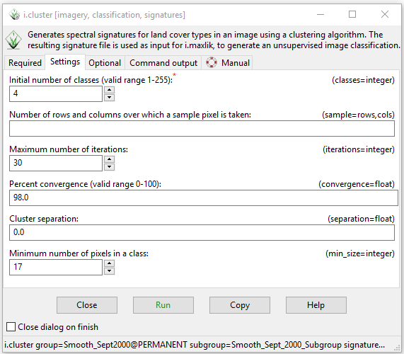 Figure 38: The i.cluster module window showing the variables available on the Settings tab.
Unsupervised Classification
i.maxlik
- 1)
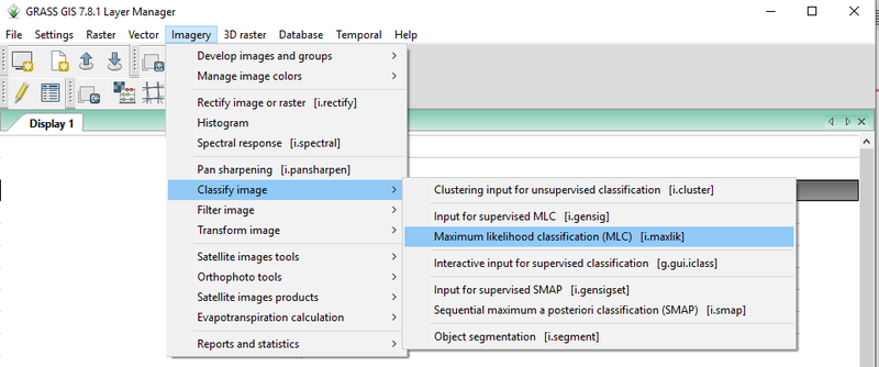 Figure 39: The path to the i.maxlik module in the Layer Manager window.
- 1)
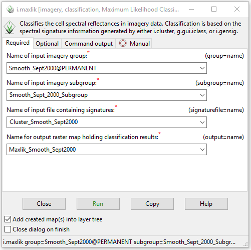 Figure 40: The i.maxlik module window showing the input and output information on the Required tab
- 1)
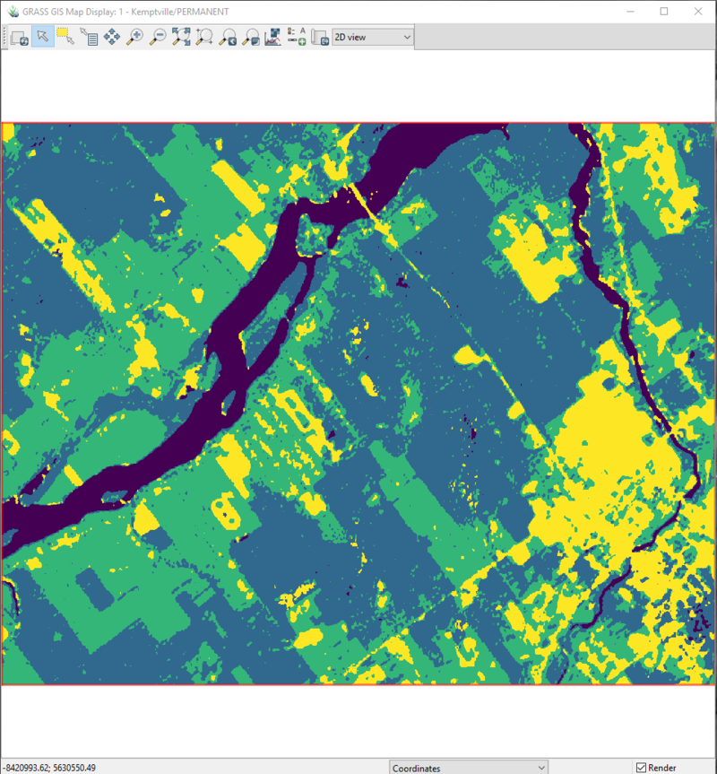 Figure 41: The classified map output for September 2000 created by the i.maxlik module.
- 1)
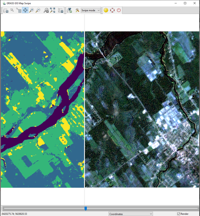 Figure 42: The Map Swipe window showing the classified imagery for September 2000 on the left, and the original imagery for bands 1, 2, and 3 for September 2000 on the right.
Landscape Change Assessment
r.change.info
- 1)
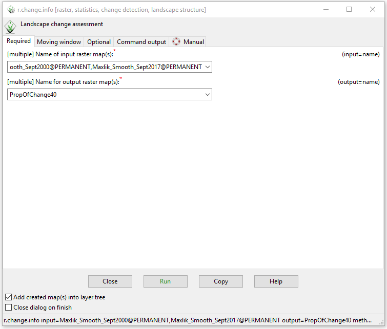 Figure 43: The r.change.info module window with the input and output information on the Required tab for the "PropOfChange40" layer.
- 1)
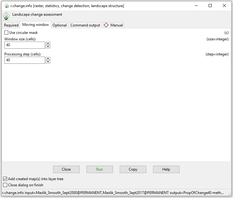 Figure 44: The r.change.info module window with variable information on the Moving Window tab, where step = 40 cells.
- 1)
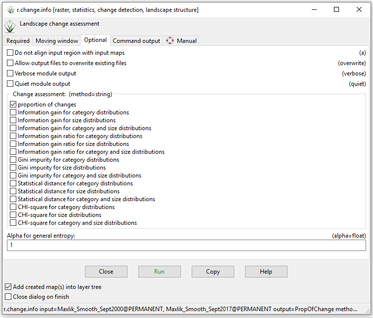 Figure 45: The r.change.info module window with the "proportion of changes" change assessment selected on the Optional tab.
- 1)
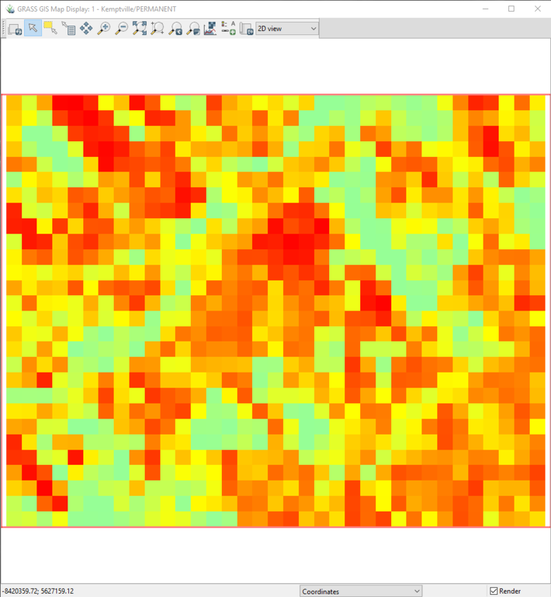 Figure 46: The output from the r.change.info module with the "PropOfChange40" layer in the Map Display window.
- 1)
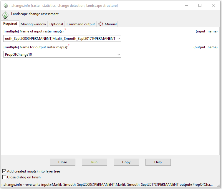 Figure 47: The r.change.info module window with the input and output information on the Required tab for the "PropOfChange10" layer.
- 1)
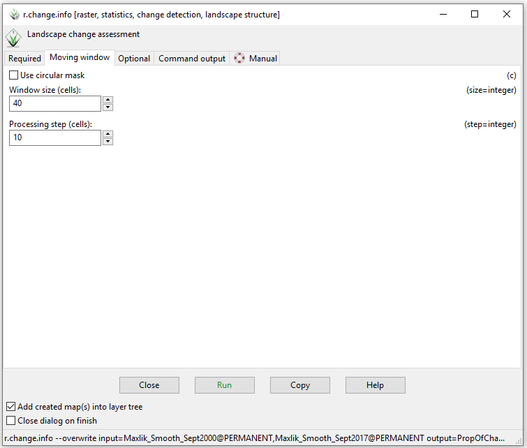 Figure 48: The r.change.info module window with variable information on the Moving Window tab, where step = 10 cells.
- 1)
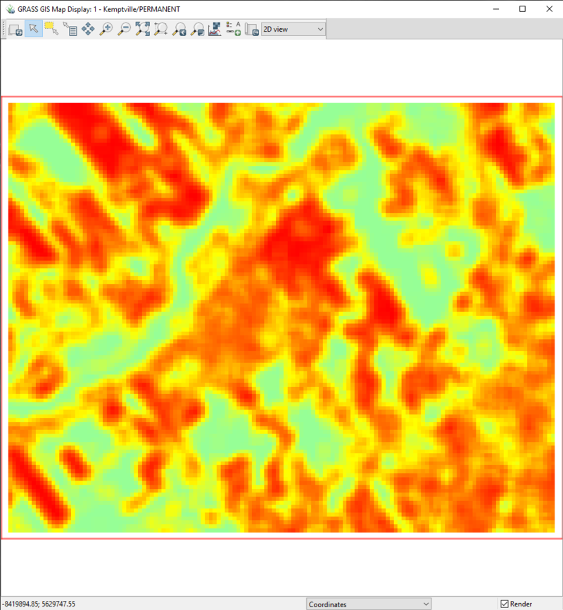 Figure 49: The output from the r.change.info module with the "PropOfChange40" layer in the Map Display window.
- 1)
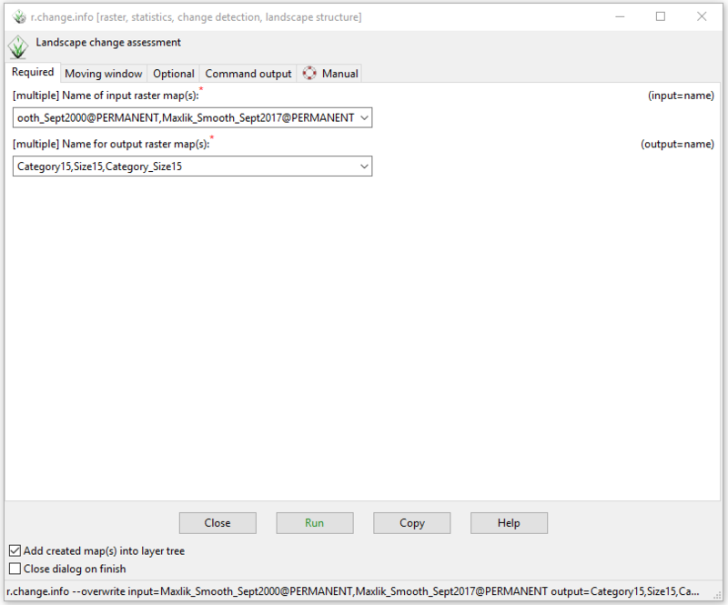 Figure 50: The r.change.info module window with the input and output information on the Required tab for the "Category15","Size15", and "Category_Size15" layers.
- 1)
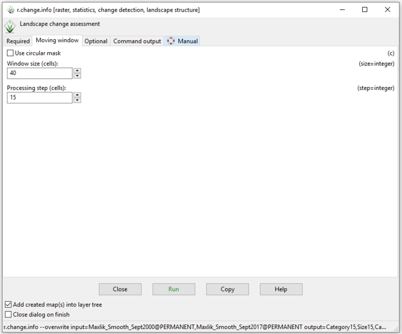 Figure 51: The r.change.info module window with variable information on the Moving Window tab, where step = 15 cells..
- 1)
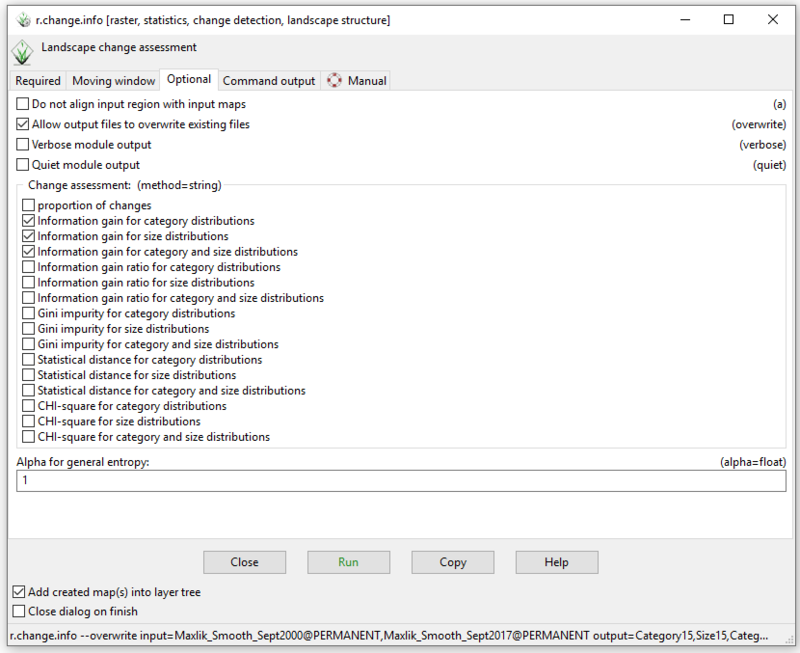 Figure 52: The r.change.info module window with "Information Gain for Category Distributions", "Information Gain for Size Distributions", and "Information Gain for Category and Size Distributions" change assessments selected on the Optional tab.
- 1)
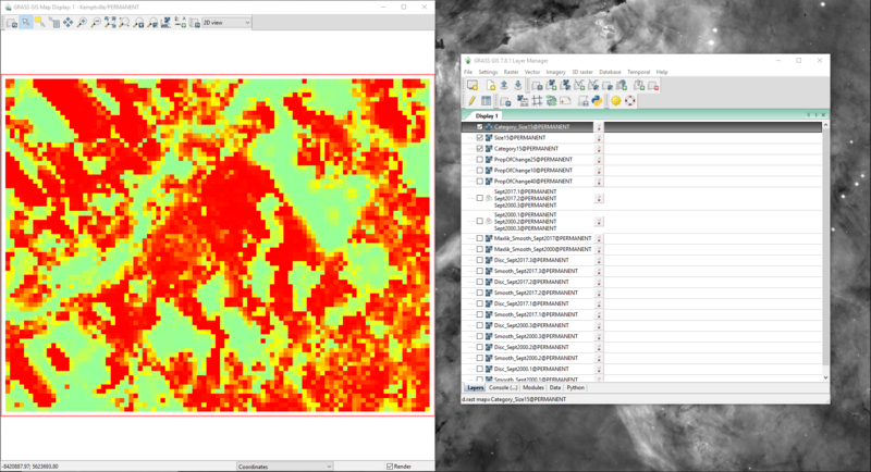 Figure 53: The output from the r.change.info module with the "Category_Size15" layer in the Map Display window.
- 1)
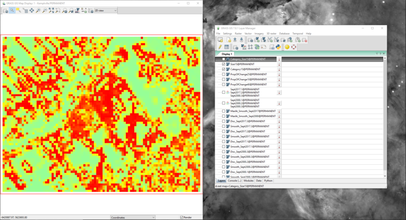 Figure 54: The output from the r.change.info module with the "Size15" layer in the Map Display window.
- 1)
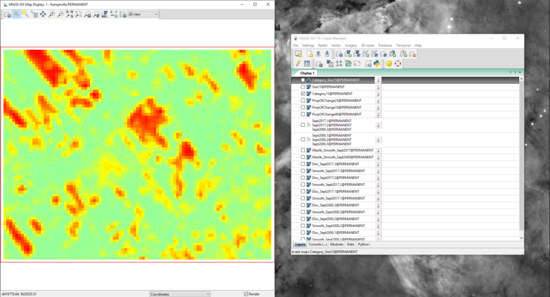 Figure 55: The output from the r.change.info module with the "Category15" layer in the Map Display window.
Editing the Landscape Change Maps for Distribution
- 1)
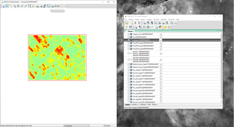 Figure 56: The "Category15" layer in the Map Display window zoomed out.
- 1)
 Figure 57: The path to the "Add Raster Legend" module (d.legend) in the Map Display window.
- 1)
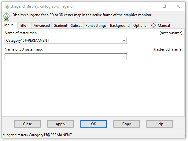 Figure 58: The Input tab in the d.legend module window.
- 1)
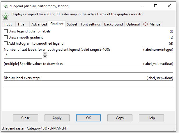 Figure 59: The Gradient tab in the d.legend module window showing where the labels for the gradient legend may be altered.
- 1)
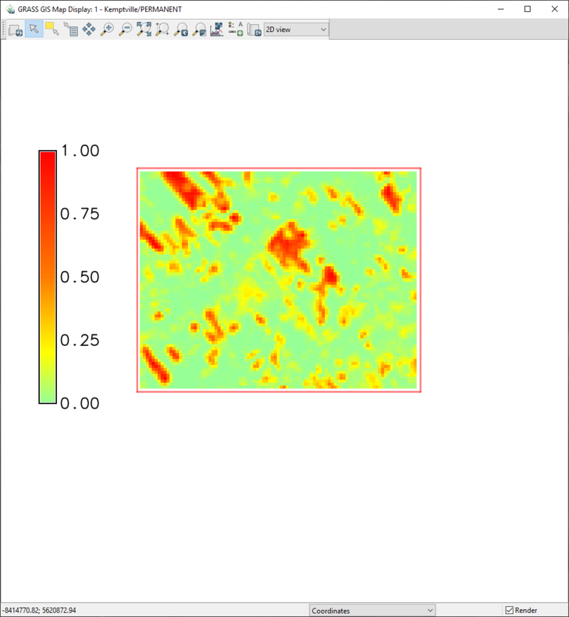 Figure 60: The "Category15" lay with a gradient legend.
Not Covered in this Tutorial
Additional Resources
Conclusion
References
https://renx.ca/kemptville-building-boom-retail-residential/
Earth Observing System (EOS) Landviewer [2]
GRASS GIS Software [3]

