R Studio’s Spatial Capabilities going 3D!

Purpose

This tutorial prominently centres on the spatial abilities of R Studio; an open software program with its own scripting language that is often used for data analysis, statistics and graphing of very large datasets. Throughout the studies of Carleton students, R Studio most likely has been used for its powerful statistical capabilities and graphing.

But the software can do so much more!

The spatial data package offers a wide range of tools that can take data and create custom maps with a myriad of customization. By no means is this package an equivalent to ArcMap or other such dedicated mapping platforms but R can do many of the same things with their own advantages.

For more about the spatial data package follow this link: https://cran.r-project.org/web/packages/sp/sp.pdf

This tutorial shows how one could create 3D maps or images using the R language – if your not familiar with R or some of its other mapping capabilities see the following tutorials;

Julia Riddick -> R Studio's Spatial Capabilities at http://gracilis.carleton.ca/CUOSGwiki/index.php/R_Studio%27s_Spatial_Capabilities

Uzayr Siddiqui -> Introducing Geoprocessing Capabilities of SAGA in R Environment using RSAGA (Saga + Rstudio) at http://gracilis.carleton.ca/CUOSGwiki/index.php/Introducing_Geoprocessing_Capabilities_of_SAGA_in_R_Environment_using_RSAGA_(Saga_%2B_Rstudio)

I'm quite fond of R & RStudio and saw how it was under represented within the tutorials over the years. The software isn't as visually 'flashy' as other platforms but much more fun to handle and manipulate at a coding level.

Objective

The objective of this tutorial is to develop the users R Studio skills, competence in the R language and to demonstrate some of the various ways that 3D maps and images can be created.

The goal is to get users thinking on how R can do more than just stats but also map. An introduction of sorts getting users to thinking beyond tables or lists and thinking in 3 dimensions.

Software Introduction

Rstudio

This is an open software program that creates a user-friendly graphic user interface for accessing the R statistical analysis and scripting language. R is often used for data analysis, statistics and graphing of very large datasets. It also has the ability to interface with the SAGA spatial analysis program, through the 69 modules shown below; users are able to use spatial data and manipulate and perform geoprocessing via special commands within this software. The more you explore and use the commands the more comfortable you will get. Initially everyone may face difficulty, however, if the basics are understood well, it eases major geoprocessing tools. R studio is known for handling large datasets with efficiency and helps in optimizing results quicker in order to perform them multiple times at a time without the needs to run through the steps again and again. Also, R not only processes data but if users may want to visualize their spatial output of their data, R has a package called sp which has that feature.

To download RStudio click the link --> https://www.rstudio.com/products/rstudio/download/

There's a great introduction on the R Studio layout and configuration found on Julia Riddick's R Studio's Spatial Capabilities at http://gracilis.carleton.ca/CUOSGwiki/index.php/R_Studio%27s_Spatial_Capabilities, so take a look and become familiar with the software.

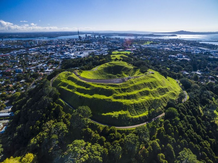
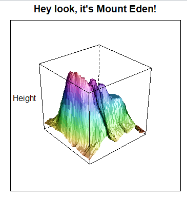
Throughout this tutorial we'll en devour to us datasets that are pre-installed in R, saving users time in tracking down data as well as for simplicity. R studio has a great volcano dataset that represents Maunga Whau (Mt Eden). This mountain is one of about 50 volcanos in the Auckland volcanic field. This data set gives topographic information for Maunga Whau on a 10m by 10m grid.

Here's what Mount Eden looks like;

The scripts that this tutorial will be using will be straight forward and simple, users will need to do some thinking on their own to wrap their heads around how to apply techniques elsewhere.

3D Mapping in a Myriad of Ways

Before doing any coding in R you'll need to think about what 'tool's' you'll need. What packages do you need to install to run any specialized functions?

Through this tutorial we'll focus on three specific packages;

plot3D for more info look here -> https://cran.r-project.org/web/packages/plot3D/plot3D.pdf

plotly for more info look here -> https://cran.r-project.org/web/packages/plotly/plotly.pdf

rgl for more info look here -> https://cran.r-project.org/web/packages/rgl/rgl.pdf

The following code will install each and 'unpack' them for use.

Using Basic Contours

The easiest way of map visualization is the use of a simple contour map.

Install the plotly package and call it in through library(plotly).

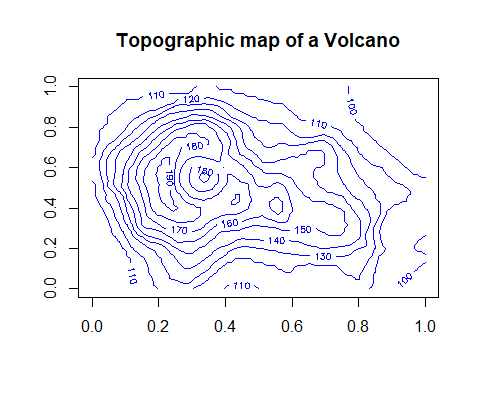
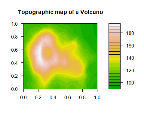
The following codes are examples of two basic ways of plotting contour maps using the aforementioned volcano dataset.

The contour line creates a basic contour map with lines in blue. See below;

While the filled.contour line creates more a complicated map with a color gradient.

It's the same data (volcano) but illustrated in two ways. This is to illustrate to you how R can make all kinds of images using your data.

Using a Lattice (Wireframe)

A straight forward method of creating a 3D image on R can be done using the Lattice package. This creates powerful and elegant graphics with minimum tuning.

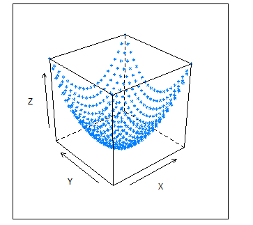
At it's most basic level what this package will do is create a 3D scatter plot (using x, y, z) and draw wires across all the points creating a 3D image.

In the context of mapping it involves using variables like the latitude, longitude and elevation to create a 3D image, akin to a DEM on Arc. Within this tutorial we're going to jump over creating custom scatter plots and use a stored dataset (volcano).

Before writing any code the lattice package needs to be installed. Clicking on the Tools tab and clicking Install Packages brings up the Install Packages Window. In the blank Packages box type in the desired package and click Install.

This will take a few seconds to successfully read in but will allow you to use all of what the package can offer.

A metaphor for what your doing by installing this packages is that you've taken the lattice tool out of your 'tool shed' (R's various packages) and put them on your 'tool belt' for access.

Here's what the code looks like.

The library(lattice); line is telling R that I'll be using some of the lattice tools from my 'belt' in this script.

The following two lines involve bring in the volcano dataset and putting the data into a matrix called cano.

The last line will do the work of creating the fictional scatter plot (you won't see it) and drap wires across the points to create the 3D imaged.

The parameters that are set will use an unclassified matrix called cano, shading the wires, telling it the aspect you want to look at it from, whether there's a title, labeling the 3 axis, and how you want to scales depicted.

This code will create the following image;

Try other parameters and see what happens. Maybe change shade = F or draw = TRUE? Changing the aspect will also change the image.

Using image2D and persp3D

Using the image2D and persp3D extension from R's image and persp function you can create 3D segments of maps, but you won't be using the scatter plot method as seen in utilizing a wireframe. First a 2D image will get generated using a default dataset and then you'll create a 3D segment from this 2D image.

Ensure that you have the necessary packages installed. Make sure you have plot3D and misc3d as they'll allow you to plot with multi-dimensional data. You can click on them in the package pane (bottom left) to get a better description.

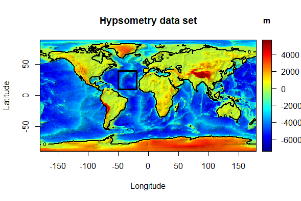
Let's create our basic map. For this you'll use the Hypsometry Data that R has built in. Hypsometry is the measurement of land elevation relative to sea level. So along that line of thought the 2D image you'll create will illustrate areas above and below sea level.

Just like creating a graph you set the parameters and labels as you see fit. The Hypsometry data is first, then we set the axis labels,explained how the contours would be set, gave it a title and a simple bar explaining the differences in the colors.

Resulting in;

This should look a bit familiar as most elevation maps look something like it. Try googling some of the areas that are red and see if they correspond with geographical phenomenon.

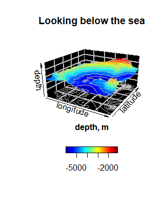
From here we'll create a 3D image using a segment of the Hypsometric data (the black square). Creating a 3D image of all the globe would use up a lot of visual space and you'd be sacrificing detail for coverage.

This 3D image illustrates a ridge/trench that runs along the sea. Where else could you apply this kind of 3D image?

Creating Composites

I've only covered a few ways of mapping in 3D but there are many more. What's really interesting is that you can bring some of the different ways of mapping together and create composites.

When you created the Bathymetric segment in the last script you also used a contour to help identify shifts in the sea level corresponding with the changing colors.

The next big step is to bring all these different ways of mapping together to create what's called a composite.