Multiple Criteria Evaluation in Allocating Land for Waste Incineration
Title should read "Multiple Criteria Evaluation in Allocating Land for Waste Incineration".
Contents
Introduction
This tutorial instructs a user in basic multi-objective decision making using a variety of Open Source software: GRASS GIS, Quantum GIS and OpenOffice Calc. With it they will be able to import vector and raster data, convert vectors to raster and use map algebra to produce a land allocation map according to the factors and constraints set up by the project. Please note that this tutorial is a followup to the GEOM4008 project proposal where we provided the context and objectives of our projects, which were not required here.
The GRASS GIS Database
In order to use GRASS software for spatial analysis a new mapset must be created to store vector and raster data. This process can be completed by a series of steps:
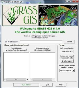
1. Open GRASS GIS and click the “Location Wizard” radio button to define a new GRASS database.
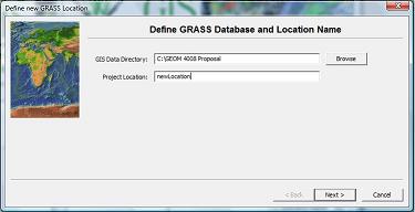
2. Choose a GIS Data Directory and Project Location, these are both folders that will be created for the database. Click “Next” to proceed to choose a method in creating the new location.
3. Select the radio button labelled “Read projection and datum terms from a georeferenced data file”. This will allow the coordinate system for the GRASS database to draw from the shapefile data included in the project, NAD83 MTM Zone 9. This is the appropriate projection and datum for the Ottawa area. Click “Next”.
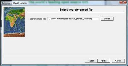
4. In the following dialogue box browse for and select any one of the shapefile data to read its projection and datum characteristics for the GRASS database. Figure 1 through 4 illustrates the creation of a GRASS GIS database.
Figure 1. GRASS welcome GUI
Figure 2. Define a GRASS database location and name
Figure 3. Choose a method of creating a new location
Figure 4. Select a georeferenced file
Import Shapefile Data to GRASS
Now that the GRASS database has been created we can import all necessary vector shapefile and raster data necessary to fulfill the project objectives. This process can completed by using the bulk import command in GRASS:
1. Navigate to the Menu Bar, select File-->Import Vector Data-->Bulk Import of Vector Data
2. In this dialogue box we can select a directory to import a set of shapefiles
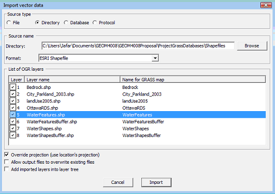
3. Select the “Directory” radio button then navigate to the projects shapefile directory as the source, select “ESRI Shapefile” as the format. Be sure to select the radio box labelled “Override projection (use location’s projection)” this will ensure that the shapefiles’ projection and datum will match the mapset. Click “Next”. Figure 5 illustrates the Bulk Import Vector Data GUI.
Figure 5. Bulk import of vector data
Feature Value Allocation
To determine the parcels of land most suitable for Waste Depots and Incineration Sites we can assign a specific cost value to acceptable and unacceptable attributes. Preparing the vector data in this manner will allow us to easily determine the placement of sites by visual inspection.
A) Feature Value Allocation: Land Use
The land use data categorizes parcels of land according to Ottawa municipal guidelines. Acceptable land use categories for this project are:
- Vacant Land
- Vacant Building
- Industrial
- Idle and Shrub Land
- Open Space
- Pits and Quarries
All other land use categories are unacceptable, acceptable categories will receive a low cost value and unacceptable categories will receive a high cost value. In order to do this we will use OpenOffice Calc program to modify the attribute database files. Although this procedure can be done using GRASS, this program consumes far less system resources to perform the same operation because it is not concerned with the spatial component of the vector data using the database.
1. Activate the OpenOffice Calc program and open the LandUse2005 database file by navigating to through the GRASS mapset directory: ProjectGrassDatabases-->newLocation-->PERMANENT-->dbf
2. A “character set encoding” dialogue box will appear, select the “Western Europe (ISO-8859-1) character set and click OK. This is the encoding that was used to produce the database file therefore we need to use it now to read them properly. Figure 6 illustrates the character set encoding GUI.
Figure 6. OpenOffice Calc character set encoding
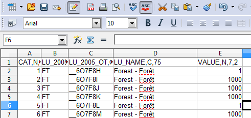
3. Now that the LandUse database file has been loaded into the spreadsheet we need to create a new column called “Value”. Do so by entering “VALUE, N, 7, 2” in the E1 cell. This will ensure that a new attribute column will be added to the vector file in GRASS.
4. To assign the proper cost values to the categories we can use a logical function that will assign “1” to acceptable categories and “1000” to unacceptable categories. In the E2 cell enter the logical function: =IF(B11="V1"; 1; IF(B11="M1"; 1; IF(B11="V2"; 1; IF(B11="ROS"; 1; IF(B11="OS"; 1; IF(B11="QS"; 1; 1000))))))
5. Migrate the function by copying the E2 cell contents and pasting it to every row in the VALUE column. Save the database file and when asked about format select “Keep Current Format”. Figure 7 illustrates the database file edit performed in step 4.
Figure 7. Using a logical function to assign values in OpenOffice Calc
B) Feature Value Allocation: Bedrock
The bedrock data contains bedrock composition and is limited to the Ottawa-Central region. We want to allocate land upon bedrock with little to no remaining economic value to other industries or to the City of Ottawa. According to the geological survey carried out by the Ministry of Natural Resources’ Mineral Resource division the Ottawa-Central region describes several bedrock types of little to no economic value:
- EASTVIEW FORMATION, DARK GREY LIMESTONE WITH SHALE BANDS
- MARCH FORMATION, INTERBEDED GREY CALAREOUS SANDSTONE & DOLOMITE.
- CARLSBAD FORMATION, GREY SHALE SOME DOLOMITE LAYERS.
- BILLINGS FORMATION
- ROCKCLIFFE FORMATION, GREY GREEN SHALE WITH GREY SANDSTONE LENSES.
- QUATERNARY FORMATION, THICK DRIFT, RECENT ALLUVIUM & PLEISTOCENE GLACIAL DEPOSITS.
To allocate values to acceptable and unacceptable bedrock types follow steps 1 through 5 of the Land Use feature allocation section but use the logical function as follows: * = IF(D2=1; 1; IF(D2=2; 1; IF(D2=4; 1; IF(D2=5; 1; IF(D2=10; 1; IF(D2=12; 1; 1000))))))
C) Feature Value Allocation: WaterFeatures
The WaterFeatures polygon vector contains data on all water features in the Ottawa region including rivers, streams and ponds. For this project, all water features will receive a high cost value of 1000 making allocation a much simpler matter than the two previous database files. To allocate values to its database table follow steps 1 through 5 but designate the VALUE cell as follows:
* =1000
This will assign a value of 1000 to every feature in the WaterFeaturesvector.
Now that each of the vectors have received an appropriate value for its features we can proceed to work with the elevation data by creating an interpolation and slope surface.
Converting Vector Data to Raster
We will use the Quantum GIS program to convert the vector data to raster; its graphical user interface (GUI) will allow us to easily change the GRASS mapset region resolution which is a crucial parameter when working with raster data (editors note: this could be done just as easily in GRASS itself). When working with raster data the GRASS mapset will refer to the resolution settings of the region, each pixel will reflect the North-South and East-West settings. To ensure optimal conversion of polygon and line vector data the resolution should be set to match the dimensions of the smallest feature, point vector data does not encounter difficulty in this process (unless points lie outside the region extent) and each point will count as the centroid for each pixel.
First we will change the mapset region resolution parameters to convert the Land Use vector data as follows: 1. Activate Quantum GIS and navigate through the Menu bar: Plugins-->GRASS-->Open Mapset. Find the primary mapset folder and click “OK” to open the mapset.
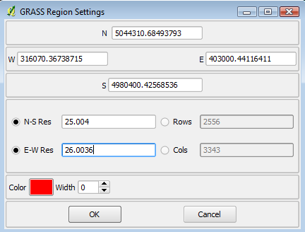
2. Edit the GRASS mapset region by clicking the icon File:Icon1.bmp. This will open the Region GUI. Figure 8 illustrates the GRASS region GUI.
3. Change the N-S Res to 25 units and the E-W Res to 25 units. GRASS uses rectangular pixels so the N-S resolution will automatically be lesser than the E-W resolution. This will instruct the raster conversion tool to create a 25m pixel per vector line or area.
Figure 8. GRASS Region GUI
Now that we have the region set we can convert the Land Use vector to raster using the GRASS “shell” command module. For each vector data we will alter the region resolution settings to reflect the vector characteristics. Open the GRASS shell module by clicking the icon ![]() and activating the shell. Figure 10 illustrates the GRASS shell module, in the shell we will enter the command to convert the Land Use vector as follows:
and activating the shell. Figure 10 illustrates the GRASS shell module, in the shell we will enter the command to convert the Land Use vector as follows:
- v.to.rast --overwrite input=landuse2005 output=LandUseRaster column=VALUE labelcolumn=VALUE
Figure 9. GRASS shell module to convert vector to raster
When the process has been completed we can convert the Bedrock vector as follows:
- v.to.rast --overwrite input=BedRock output=BedRockRaster column=VALUE labelcolumn=VALUE
Before we convert the WaterFeatures vector to raster we must apply a buffer to it. No Incineration Facility or Waste Depot should be constructed within 300 metres of any body of water. The most efficient way to do this is to alter the Region settings to 5m resolution and use the v.buffer tool to place a buffer around the WaterFeatures vector. Using the GRASS shell input the command as follows:
- v.buffer input= WaterFeatures output= WaterFeatures Vector --overwrite type=area layer=1 distances=300 tolerance=0.1
This will create a new vector with round polygons. Now we can convert that vector to raster as follows:
- v.to.rast --overwrite input= WaterFeatures Vector output= WaterFeaturesRaster column=VALUE labelcolumn=VALUE
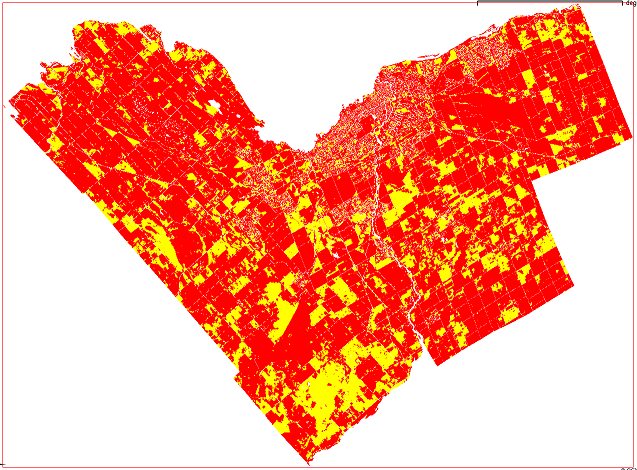
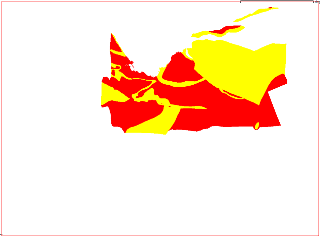
In this manner we have created three separate rasters. The LandUseRaster and BedRockRaster each contain 2 pixel classes: 1 and 1000 to indicate acceptable and unacceptable land respectively. The WaterFeaturesRaster contains only 1 pixel class because its buffered zone indicates only unacceptable areas for construction. It is important to make note that the rasters were created with NULL values where no pixel received a value due to the vectors’ extents. In the final land allocation process we will use GRASS’s map algebra tool to combine the rasters and so their NULL values must be accounted for. Figures 10 through 12 illustrate the WaterFeatures, LandUse and Bedrock rasters.
Figure 10. WaterFeatures Raster
Figure 11. LandUse Raster
Figure 12. Bedrock Raster
Land Allocation Using Map Algebra
=Dealing with NULL Values To deal with the NULL raster values we can use the r.null tool in the GRASS shell to assign a value of 0 so they can be recognize by map algrebra but do not participate in the combination process:
- r.null map=WaterFeaturesRaster null=0
- r.null map=BedRockRaster null=0
- r.null map=LandUseRaster null=0
These commands will create a separate class for null values in the system memory and will appear visually as a different colour.
Using Map Algrebra to Allocate Best Area for Incineration
Now that we have the 3 rasters we can use map algebra to create a Land Use Suitability Map that should indicate the maximum area for use by Incineration Facilities and Waste Depots. When the suitability map has been created we can return the map NULL values to NULL instead of 0 so that only the relevant areas are shown.
1. WaterFeatures Raster contains two pixel values in addition to the null values: 1 and 2. We must use map algebra to reduce both classes to a value of 1 then convert them back to their original cost value of 1000.
2. In the GRASS shell enter the following commands to return WaterFeaturesRaster to a single high cost value:
- r.mapcalculator –overwrite formula=(oldraster^0)*1000 outfile=WaterFeaturesA
3. Then we use map algebra again to create the Land Use Suitability Map
- r.mapcalculator --overwrite formula=WaterFeaturesA+ BedRockRaster + LandUseRaster outfile=LandUseSuitabilityMap
4. Now that the Land Use Suitability Map has been created we can convert the null values back to zero:
- r.null map=LandUseSuitabilityMap setnull=0
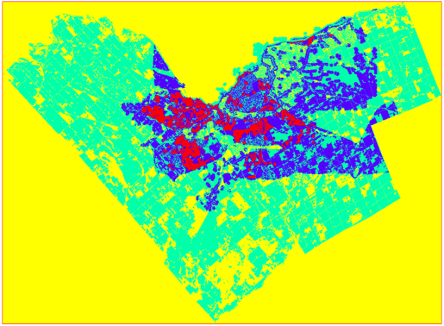
Figure 13 illustrates the output LandUseSuitabilityMap from the map algebra process.
Figure 13. LandUseSuitabilityMap
The output raster contains four different pixel classes. In order to approximate the real world land-use allocation we can convert the raster to vector then use QuantumGIS’s superior symbology system to differentiate between acceptable and unacceptable land.
1. Using the GRASS shell enter this command to convert to vector:
- r.to.vect -s -v input=LandUseSuitabilityMap output=LandAllocationMap feature=area
2. Add the output vector to the QuantumGIS map space and open the symobology settings by right-clicking the vector and selecting “Properties”.
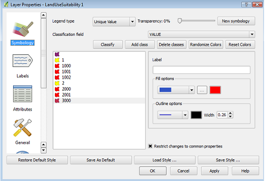
3. In the “symbology” tab set the Legend Type to “Unique Value” and Classification field to “VALUE”, click the Classify radio button.
4. Now we see that several classes have been created as a result of the map algrebra, recall that we had set acceptable land allocations to a value of 1 and unacceptable land allocations to 1000. Due to the map algrebra process acceptable values will have a maximum value of 2 indicating areas of appropriate land use and bedrock type as well as being at least 300m away from any body of water.
5. De-select the radio button “Restrict changes to common properties” and assign like colours to values 1 and 2 and like colours to the remaining classes. This will ensure a clear land allocation vector for visual inspection.
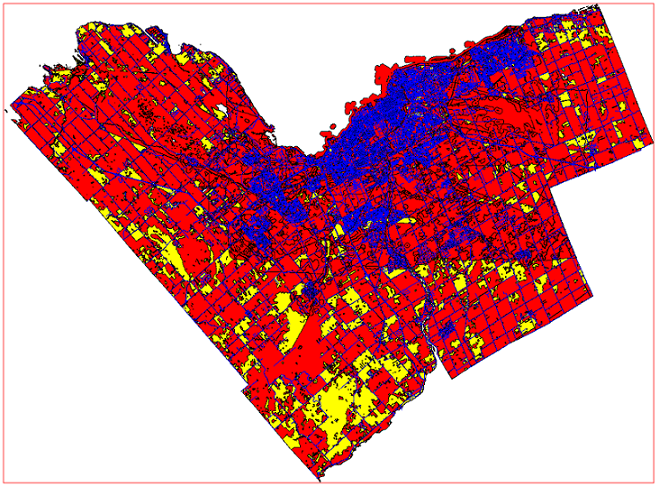
Figure 14 illustrates the symbology GUI for the Land Allocation Map. Figure 15 illustrates the Land Allocation Map with two classes yellow representing suitable land allocations and red representing unsuitable land. The black areas represent remnants of the nodata process when converting from raster to vector. The Ottawa Transportion Data (roads) vector data has been added to the mapset and Incineration Facilites and Waste Depots can be positioned appropriately to serve different communities in an optimal fashion.
Figure 14. GRASS symbology GUI
Figure 15. Land Allocation Map
Conclusion
This tutorial instructed the process of using vector data to determine land allocation according to several factors and contraints, the result being a Land Allocation Map showing areas appropriate for Incineration and Waste Depots. We used several GRASS and Quantum GIS tools to carry out project objectives as well as OpenOffice Calc which played an important role in assigning cost value to land parcels.
Quantum GIS functioned primarily as a visual aid when using its bundled GRASS toolset to manipulate the symbology of vector and raster data, its graphical user interface (GUI) being far easier to navigate. While GRASS functionality is bundled with Quantum GIS both were used individually depending upon what phase of the project I was in and the specifications of the computer I was using. GRASS GIS was intended to perform the bulk of the data processing tasks for this project. OpenOffice’s Calc program is the Open Source version of Microsoft Excel and it played an important but brief role in fulfilling my project objectives: assigning feature value. Microsoft Excel 2007 does not support the edit of database files (a deprecated functionality) therefore it was all the more sensible to use an open source software that could do the job and Calc did the job well.
References
- GRASS GIS Version 6.4.0 available here: (GRASS GIS)
- Quantum GIS Version 1.5.0 available here: (QGIS)
- OpenOffice Calc available here: (OpenOffice )
- Fraser, John Z. (1976). Mineral Resource Survey. In DIVISION OF MINES, GEOLOGICAL BRANCH Open File Report 5217. Retried November 25, 2010 from
