Landscape Structure Analysis Using the Landscape Patch Analysis Toolset in GRASS GIS

Introduction to Landscape Patch Analysis

Landscape Ecology

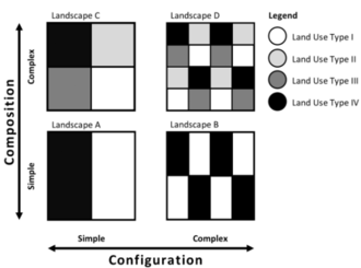
Landscape ecology is the field of study concerned with determining the spatial patterns and spatial pattern change in terms of landscape structure. Landscape structure refers to the organization of the landscape in terms of its spatial heterogeneity. There are two aspects of spatial heterogeneity that we can examine through landscape structure analysis; composition and configuration. Composition refers to the different elements of a landscape. Configuration refers to the spatial arrangement of the elements, see Figure 1.

Figure 1. A diagram explaining the difference between composition and configuration in the context of landscape ecology. (Gehrke and Clifton, 2017)

Based on these elements, spatial heterogeneity or homogeneity can be construed by examining patches in the structure statistically.

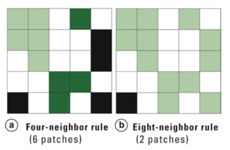
Figure 2. A diagram depicting the four-neighbor vs. eight-neighbor rule for defining landscape patches. (Turner and Gardner, 2015)

Patches are areas of connected homogeneous land cover; they can be examined for spatial patterns and statistical measures which are telling of structure. The landscape can then be evaluated in terms of the impact of structure on ecological phenomenon and ecosystems. Patches can be defined using either the four-neighbor rule or the eight-neighbor rule, see Figure 2. The four-neighbor rule defines patches as areas that are connected by pixels in only the four orthogonal directions. This results in smaller patches but a greater number of patches overall. The eight-neighbor rule defines patches as areas that are connected by any of the eight pixels that surround a given pixel. This results in larger continuous patches but a fewer number of patches overall. This is one of the many decisions a researcher can make which may impact the results of a landscape structure study.

The value in examining the configuration and composition of landscapes is to have a greater understanding of the factors influencing ecosystem health in a statistically valid way, awareness of possible detriments to species, and the ability to examine patterns in a given landscape at varying degrees of complexity. Examining landscapes at varying grains and extents can have an impact on the results of a study. Grains that are too coarse to show smaller patches could result in misinterpretation of the landscape, or this may be done purposefully to reduce complexity. Deciding on extent can be difficult because ideally you would not want to artificially divide a landscape patch due to the placement of the boundary for the study as this produces false information about metrics such as mean patch size and edge density.

Methods in Landscape Structure Analysis

Landscape ecology methods in this tutorial will include several of the options provided in the landscape patch analysis toolset in GRASS GIS. This should provide a solid background for the steps involved in using tools from this kit and provide an introduction to landscape ecology metrics. Later on in this tutorial the results of these metrics will be briefly interpreted to explain the structure of the landscape and provide the reader with a sample of an elucidated landscape.

Mean Patch Size

Mean patch size is the average number of pixels the patches in the landscape contain. Most landscape metrics use patch size information or are affected by patch size. This is a very simplistic spatial attribute to examine in the landscape. This would be directly affected by the users choice of four or eight neighbor patch definition, and therefore affect many of the other metrics.

Patch Number

Simply the number of patches defined in your landscape. This will be directly impacted by the patch rule that is chosen.

Patch Density

This is the number of patches, continuous areas of homogeneous land cover, per unit of area in the landscape. This would change depending on whether the four-neighbour or eight-neighbour rule was used.

Edge Density

Edge density can be calculated for all patches or for a particular patch type. It is the length of edge per area of the patch.

Figure 3. A visual explanation of edge density between forested and urban patches. (Turner and Gardner, 2015)

Simpson's Diversity

A Note About Executing Commands in GRASS GIS

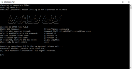
All commands in GRASS can either be executed by navigating through the menus and opening GUIs or by typing into the command shell, see Figure 4. This tutorial will walk the user through the steps using the GUIs because this is a more intuitive user interface and suits all individuals, including those who are not comfortable with coding.

If you wish to execute commands in the command shell, the commands for each step appear in brackets beside the function as you navigate though the menus.

Figure 4. The command shell for grass where processes can be executed by typing the appropriate coded instructions.

Data for Tutorial

Please download a satellite image over a small area of interest. Please select an area with simple land cover types which are easily separable, such as water, forest, and exposed soil.

Free satellite imagery can be acquired from site such as Landviewer (https://eos.com/landviewer/?lat=43.6591&lng=-79.4626&z=11), the USGS Earth Explorer (https://earthexplorer.usgs.gov/), and the Sentinel Hub (http://apps.sentinel-hub.com/eo-browser/). Save your file as "ClassifiedImage".

The satellite image file used in this tutorial was downloaded from Landviewer, it is a Sentinel 2A image over Bobcaygeon, Ontario.

Landscape structure analysis is performed on classified data, so first we will quickly go over how to run an unsupervised classification on the image.

Figure 5. The Sentinel-2 image of Bobcaygeon, Ontario obtained through Landviewer.

Tutorial Methods

Starting up GRASS GIS and Setting up the Database

Launch GRASS GIS 7.6.1 from your desktop.

If you are starting GRASS GIS for the first time on your computer you may see a notice appear addressing this. Select "OK" when you have read it.

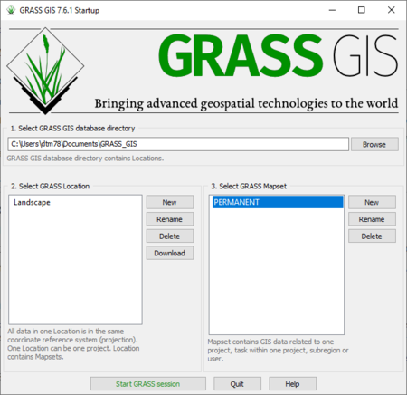
GRASS requires that a database be created where files can be stored in a GRASS-specific hierarchy formats. The GRASS GIS 7.6.1 Startup window prompts you to set up a database directory. See Figure 4.

Figure 6. Startup window for GRASS GIS 7.6.1.

In the first section, create and browse to a folder called "GRASS_GIS".

In the second section, create a new location by selecting "New" and name the location "Landscape". Select "Next".

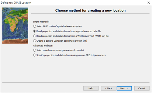
The data in this location will all use the same spatial reference system; which you specify in the this window. Choose the option "Read projection and datum terms from a georeferenced data file", see Figure 5.

Figure 7. Select the method of determining the spatial reference system in this window.

Select "Next" and in this window navigate to the location where the satellite image you downloaded is saved. Select the image file. Select "Next", then "Finish". Select "Yes" when prompted as to whether the selected layer should be imported into the database. If this does not work, and the file is not automatically imported, a method of manually importing the image will be executed in the next section.

In the GRASS GIS 7.6.1 Startup window, single-click the "Landscape" location and single-click on "PERMANENT" in the third section.

Select "Start GRASS session".

Importing the Satellite Image

To import the satellite image for classification, navigate through the following menus to open the GUI for raster import.

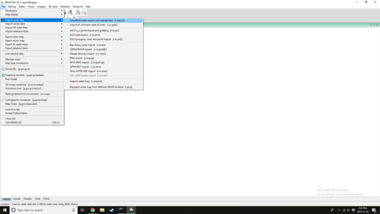
File > Import raster data > Simplified raster import with reprojection [r.import]

Figure 8. Importing a raster layer.

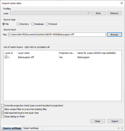
The GUI will open. Select the satellite image you downloaded.

Figure 9. GUI for importing a raster layer. Select your satellite image in this window.

Creating an RGB Image

To create a RGB colour composite image, navigate through the following menus to open the GUI for creating RGB images.

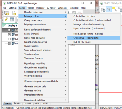
Raster > Manage colours > Create RGB [r.composite]

Figure 10. Creating an RGB composite.

References

http://www.umass.edu/landeco/teaching/landscape_ecology/labs/neutral.lab3.pdf
https://www.glel.carleton.ca/RESEARCH/landsecol.php#Landscape%20Ecology
Gehrke, S. R., and K. J. Clifton. 2017. An activity-related land use mix construct and its connection to pedestrian travel. Environ. Plan. B Urban Anal. City Sci. 46: 9–26.
Turner, M. G., and R. H. Gardner. 2015. Landscape ecology in theory and practice: Pattern and process, 2nd ed. Springer New York.