Spatial data and analysis in R using terra
Spatial analysis and the handling of spatial data have long been powerful capabilities in R. However, recently the dominant libraries providing these capabilities (including sp, raster, rgdal, ...) have been declared obsolete and were removed from current versions of R. New replacement packages include terra and sf. This move has advantages in that it removed a mix of incompatible tools, forcing standardization, and boosting the ability to use larger, modern datasets. It does mean, however, that there are a lot of tutorials and other documentation on the Internet or in books about spatial data analysis which is now also out of date.
This tutorial aims to help fix that situation. In the spirit of most of the tutorials on this site, it will use only open data, and while we focus on data centred on Carleton University, the same methods should work on similar data from anywhere else in the world. It was developed using R-4.3.1, and I am running it within the RStudio environment, which will show up in screenshots, and there are a few setup instructions given that are specific to RStudio. Besides that, the actual processing will be demonstrated using just console-based R commands, so they should work in any R environment.
This is written assuming that you have general computer / file management skills. We don't assume you already know how to use R, but we also don't go out of our way to explain it. A good general introduction is available at the RSpatial site (click here). We also assume that you already know some basics of spatial data, such as what is meant by vector and raster data, projections, and coordinate reference systems.
Contents
Get data
To start with, we need some data. On your computer's local storage / hard drive, please create a new folder where you will store everything related to this exercise.
First, we will use some Landsat imagery, from the open archive provided by USGS.
To speed things up, I used Google Earth Engine, to take advantage of their huge collection of open data and their tools so I could quickly search for images free from cloud cover, and clip then export an image surrounding Carleton University. Here's a short tutorial on how to make use of Google Earth Engine to look for and download imagery. As long as you pick an area that includes some version an area centred on downtown Ottawa or the region around Carleton University, the rest of this tutorial should work. While you are in Google Earth Engine, please take note of the unique identifier (ProductID) of the image that you obtain - you can do that by looking at the metadata printed to the console when you run the script in the tutorial. In my example, I obtained the GEE id LANDSAT/LC08/C02/T1_L2/LC08_015029_20190508; the last part of that (starting with LC08, is the ProductID.
However, if you're in a rush and want to stay focused on R, the file lined here contains an image I have already exported in GeoTIFF format.
Next, we will get some vector data from the City of Ottawa Open Data; there's a lot there you can explore, but to get started, we will download Parks and Greenspace data and Ottawa Neighbourhoods into the same folder you used above. Extract the contents of any .zip files.
Start R using RStudio and set environment
Launch RStudio on your computer (e.g. on a Windows computer, find it on the Start Menu; on a macOS computer, it's probably in your Applications folder). On the File menu, choose New Project. Choose the Existing Directory option, and then point it to the directory where you saved your data files, above. You should then have a blank RStudio project, set to use your data directory as the working directory for all work in R (you could use the getwd() command to double check this).
Try loading the Terra library (we will discuss more on what this does below) by typing the following at the prompt in the RStudio Console, and pressing Enter:
library("terra")
If you get an error stating that the library was not found, you will need to install it in the local library collection on your machine, using the following command:
install.packages("terra")
That should download and install the library, so that it will be available for you from then on if you return to this same computer.
About the Terra library
When you loaded the Terra library, it added a number of classes to the R environment that support spatial data, and functions to access, analyze, and visualize those data. The data class SpatVector holds vector data, and SpatRaster handles raster data (for more details, see RSpatial's documentation of SpatVector and SpatRaster). When I wrote that SpatRaster "handles" raster data I chose that verb carefully - an important advance in raster data handling compared to some older libraries is that the data do not have to all reside inside the R data library - R typically holds all of its active data objects in the computer's working memory. Raster grids can be very large, so loading all the raster files you are working on into the computer's active memory can quickly fill it up; instead, it is much more efficient to keep the raster data on your storage device (hard drive, network drive, etc.) and just access parts of the grid as needed. SpatRaster objects CAN have data stored within them, but in the majority of "real life" cases, most of the data stays in external files and the R data object holds metadata like the coordinate reference system being used, the bounding coordinates and resolution of the grid, etc.
Reading spatial data into R
To load in the satellite image, use the following command at the R command prompt. Note that one thing that the RStudio development environment provides on top of basic R capabilities is things like command completion prompts. When you start typing the first few letters of a data object or function name, hit the tab key, and a list of potential matches to what you have entered appears; once you see the one that matches, you can just choose it (with the mouse or the up / down keys on the keyboard) instead of typing the whole name in. Similarly, once you open the brackets at the end of a function name, you can use the same completion mechanism to put R objects in as parameters to the function.
rawImage <- rast(choose.files())
The choose.files() function will cause the RStudio gui to pop up a window that lets you navigate to and select the input file, which in this case is "LC08_1629863183191865.tif" - note that alternatively, you could have typed that file name (with quotes) in as the function's argument.
Now import the vector data:
roads <- vect(choose.files())
and then choose the file (I downloaded shapefiles, so chose the file ending in .shp; adjust as needed for the file format you chose).
And the same for the neighbourhoods data:
nbrhds <- vect(choose.files())
Investigating the data
Now let's take a look at what we've imported. Enter just the name of our image at the R command prompt (and press Enter):
rawImage
You should see output something like:
> rawImage
class       : SpatRaster
dimensions  : 237, 463, 19  (nrow, ncol, nlyr)
resolution  : 30, 30  (x, y)
extent      : 441405, 455295, 5020935, 5028045  (xmin, xmax, ymin, ymax)
coord. ref. : WGS 84 / UTM zone 18N (EPSG:32618)
source      : exportedImage.tif
names       : SR_B1, SR_B2, SR_B3, SR_B4, SR_B5, SR_B6, ...
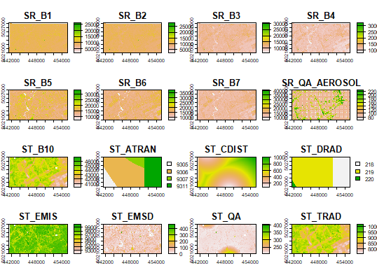
Let's look at the images. If you simply enter the following command, R will cram each band into the output plot window:
plot(rawImage)
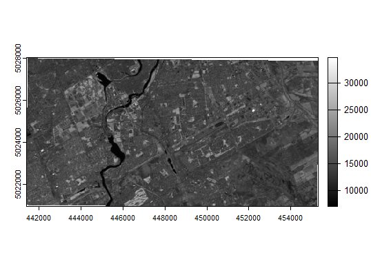
If you wanted to look at just the NIR band, using 255 shades of grey, you could use this:
plot(rawImage$SR_B5, col=gray(0:255 / 255))
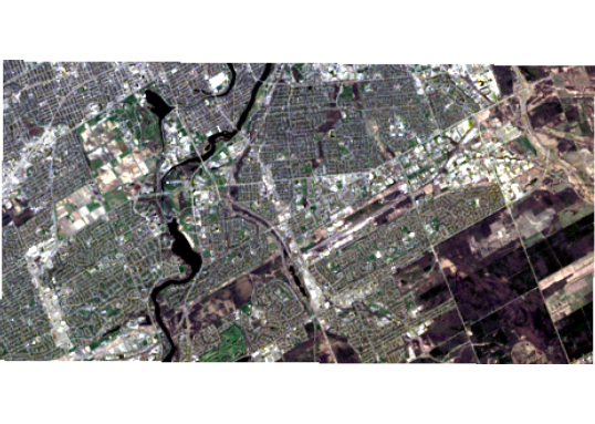
How about a visual composite (assigning the "true colour" red, green, and blue measurements to their respective colours on the display)?
plotRGB(c(rawImage$SR_B4, rawImage$SR_B3, rawImage$SR_B2), stretch="lin")


