Determining Effects on Temperature Interpolations from Large Lakes using QGIS

Introduction

Purpose

The purpose of this tutorial is to provide a guide for creating an Inverse Distance Weighting (IDW) interpolation in GRASS GIS, and analyzing the spatial errors produced in interpolated data by large interrupting features. This tutorial will aim to create a usable set of layers in QGIS, including an Ontario shapefile, an Ontario lakes shapefile, and a point vector layer of temperature data collected at climate stations in Ontario. Next, the guide will demonstrate how to use these layers to create an IDW interpolated raster layer for temperature using GRASS GIS. Finally, _____________________________________________________ in order to analyse the errors produced in the interpolation.

Background Information

An Inverse Distance Weighted (IDW) interpolation follows Tobler's First Law of Geography; near things are more alike than things that are farther apart. IDW uses the values surrounding the location of interpolation to a certain distance and assigns weighting factors to them. Values that are closer to the area being predicted have more weight in predicting the value than values that are further away. IDW interpolation is sensitive to outliers.

In Canada, the Great Lakes are key geographic features whose effects are as strong as to create a weather phenomenon that impacts the temperature of neighboring land regions. The concept of lake-effect is that large bodies of water are slow to react to changes in temperature; they stay warmer for longer in the winter than the temperature on land, and they remain cold well into the spring. For this reason, locations that border large lakes, such as the Great Lakes and the world oceans, have their temperature moderated by the movement of warm or cool air off of the bodies of water. Lake-effect also causes variations in moisture over nearby land masses leading to coastal weather being very unique.

This project has additional uses outside of lake-effect as well, as you could analyze errors in temperature interpolation caused by urban heat islands, or errors in interpolation caused by other types of large geographic features that relate to geospatial phenomenon like weather.

Software

The software used for this project was QGIS, GRASS GIS, and ___________, which are free and open-sourced GIS software.

The software can be downloaded here: https://www.qgis.org/en/site/forusers/download.html for QGIS and https://grass.osgeo.org/download/ for GRASS GIS.

QGIS was used to set up the data into a usable form (i.e. correct projection). GRASS GIS was then used to create the interpolation and data extraction for further interpretation. ____________ was used to analyze the data and examine the spatial error.

Data

The data used in this tutorial includes a shapefile of Ontario, a shapefile of lakes within Ontario, and temperature data for climate stations in Ontario represented as points. In this tutorial there will be two examples completed; one using data from a date in spring (the area beside the lake should be cooler than everywhere else) and one using data from a date in late fall (the area beside the lake should be warmer than everywhere else). The data can be found _______________________________________________________.

This tutorial will work for any point values wanted to use for interpolation.

Tutorial

Loading the Data in QGIS

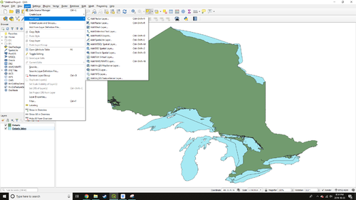
After installing the software the first thing that needs to be done is to upload the Ontario and Ontario lakes data into the program. Use the Add Vector Layer, as the data is in vector format. (Layer/Add Layer/Add Vector Layer) See the image below to navigate to this step.

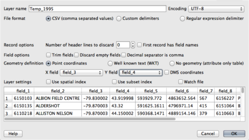
To add the temperature point data use Add Delimited Text Layer instead of the Add Vector Layer. (Layer/Add Layer/Add Delimited Text Layer) Add the file from your data, and select CSV for the file format (Note: Make sure the table file is set as CSV). For this file, there should be no header checked, and fields 3 and 4 are used for X field and Y field respectively. See the image below to navigate to this step.

Note: It is wise to keep all needed data in one folder, and save all of the produced data to the same folder as well.

Interpolation in GRASS GIS

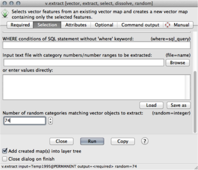
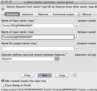
Now that the data are imported and in the proper format, we can add them to GRASS GIS for the interpolation methods. This is done (similarly to QGIS) using the add vector tool in GRASS. When the data are uploaded, we first need to separate the 1995 temperature points into validation and training sections to use. This is done using the select by attributes function (Vector/Feature Selection/Select by Attributes). In this tutorial, we used 20% points for validation, and 80% for training. Select the Temp1995 file for input, and label your output points for the validation. On the next tab (Selection), scroll to the bottom and put 20% of the points in the box (I used 74). Next, the temperature data needs to have the training points separated (Vector/Feature Selection/Select by Another Map). Use your Temp1995 for the ainput, your validation file for the binput, label the output, and select disjoint for the operator. This will create a new file for the training points.

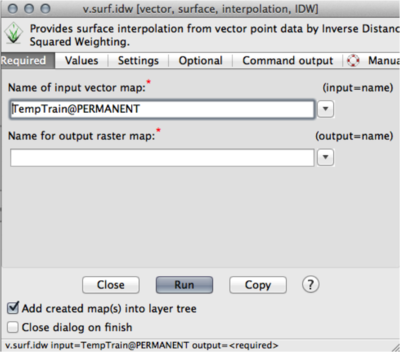
The interpolation can now be executed using the IDW from Vector Points (Raster/Interpolate Surfaces/IDW from Vector Points). Select your training data for the input vector map, and label the output as your IDW. The values should be the temperature values (Field 11 for this example). The remaining fields can be left at default, and the interpolation can be run.

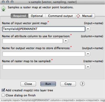
You can now use the validation points to cross-validate the interpolation. This can be done using the Sample Raster Neighbourhood Around Points (Vector/Update Attributes/Sample Raster Neighbourhood Around Points). Select the validation points as the input, the temperature data for the column, the IDW for the raster, and label the output.

The distance between the validation points and the nearest lake will need to be known, and can be found using Nearest Feature tool (Vector/Nearest Features). Select the validation points for the first input, (from tab) and the final_lake for the second input (to tab).

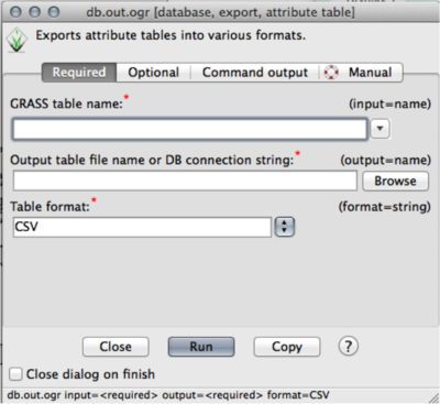
Finally the data can now be extracted to a table format to be used for analysis by using (File/Export Database Table/Common Formats Using OGR). Use your output from the previous method as the input and dsn, and format as CSV.

Analysis

The resulting CSV can now be analyzed using a variety of programs (R, excel, etc.) that can create graphs and figures. Graphing the distance on the x axis and the Mean Bias Error (validation value - interpolated value) can show the magnitude of the errors (increasing away from zero) as you move farther from the lakes. This can be accomplished better by doing multiple interpolation and analyses, as this will solidify the accuracy of your assessment (ie. the law of big numbers). Attached is a sample graph showing my results from multiple interpolations (not shown in the tutorial, but useful for reference).

Conclusion

This tutorial focuses on a feature's effect on interpolation error, and is not specific to only lakes and temperature. This has a wide range of applications throughout many different scenarios. The use of multiple programs simplifies some of the difficulties within the programs, but adds extra steps in the process. The tutorial produces an effective way to assess how proximity to a feature influences the interpolation errors.