Determining Effects on Temperature Interpolations from Large Lakes using QGIS
Contents
Purpose
The purpose of this tutorial is to provide the steps necessary for creating an Inverse Distance Weighting (IDW) interpolation in QGIS, and how to analyze the errors generated spatially. More specifically, you can interpret these errors with proximity to features in question (large lakes in this project) to see how the distance to a lake affects the error in the interpolation.
Introduction
An Inverse Distance Weighted (IDW) Interpolation uses surrounding known points (i.e. elevation) to estimate point values across an area, using the known points values. The IDW takes the distance away from the surrounding points to determine the estimated values. With the creation of this IDW interpolation, error is created because the interpolation is only estimated values across the area. It is known that lakes have a moderating effect on temperature, and so this project seeks to assess the impact on error of interpolations, rather than on temperature. This project has unlimited uses outside of lake effect as well, as you could analyze urban areas, forests, or any other type of feature/land type and its effect on quantitative values.
Software
The software used for this project was QGIS, which is a free and open-sourced GIS software. This tutorial was completed on Mac OS X, but will work with other operating systems as well. The software can be downloaded here https://www.qgis.org/en/site/forusers/download.html
Data
The data used in this tutorial includes a shapefile of large lakes within Ontario, a shapefile of Ontario, and temperature data for Ontario represented as point data. The data used can be found freely online to use in QGIS, and this tutorial will work for any point values wanted to use for interpolation.
Tutorial
Adding Data
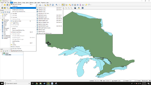
After downloading the QGIS with the link posted above, the first thing that needs to be done is uploading the data into the program. This can be done by using the Add Raster Layer or Add Vector Layer tools, depending on the type of data being used. For the case of this specific project, the data is in vector format (polygons) and the vector tool will be used. (Layer/Add Layer/Add Vector Layer)
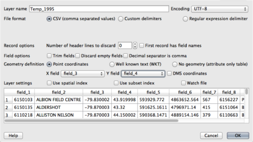
To add the point data (temperature) you will need to use the Add Delimited Text Layer instead of the Add Vector Layer (Layer/Add Layer/Add Delimited Text Layer). Add the file from your data, and select CSV for the file format (Note: Make sure the table file is set as CSV). For this file, there should be no header checked, and fields 3 and 4 are used for X field and Y field respectively.
Note: It is wise to keep all needed data in one folder, and save all of the following data to the same folder as well.
Interpolation
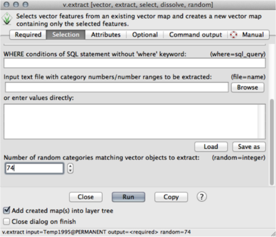
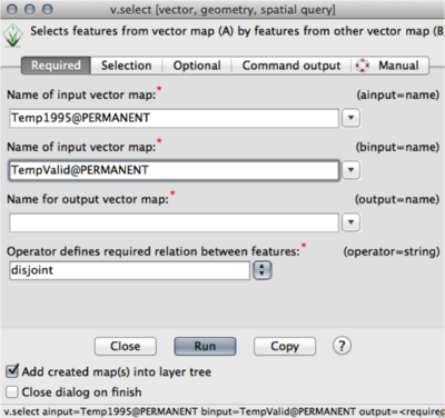
Now that the data is imported and in the proper format, we can add it to GRASS GIS for the interpolation methods. This is done (similarly to QGIS) using the add vector tool in GRASS. When the data is uploaded, we first need to separate the 1995 temperature points into validation and training sections to use. This is done using the select by attributes function (Vector/Feature Selection/Select by Attributes). In this tutorial, we used 20% points for validation, and 80% for training. Select the Temp1995 file for input, and label your output points for the validation. On the next tab (Selection), scroll to the bottom and put 20% of the points in the box (I used 74). Next, the temperature data needs to have the training points separated (Vector/Feature Selection/Select by Another Map). Use your Temp1995 for the ainput, your validation file for the binput, label the output, and select disjoint for the operator. This will create a new file for the training points.
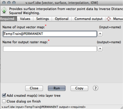
The interpolation can now be executed using the IDW from Vector Points (Raster/Interpolate Surfaces/IDW from Vector Points). Select your training data for the input vector map, and label the output as your IDW. The values should be the temperature values (Field 11 for this example). The remaining fields can be left at default, and the interpolation can be run.
You can now use the validation points to cross-validate the interpolation. This can be done using the Sample Raster Neighbourhood Around Points (Vector/Update Attributes/Sample Raster Neighbourhood Around Points). Select the validation points as the input, the temperature data for the column, the IDW for the raster, and label the output.
The distance between the validation points and the nearest lake will need to be known, and can be found using Nearest Feature tool (Vector/Nearest Features). Select the validation points for the first input, (from tab) and the final_lake for the second input (to tab).
Finally the data can now be extracted to a table format to be used for analysis by using (File/Export Database Table/Common Formats Using OGR). Use your output from the previous method as the input and dsn, and format as CSV.
Analysis
The resulting CSV can now be analyzed using a variety of programs (R, excel, etc.) that can create graphs and figures. Graphing the distance on the x axis and the Mean Bias Error (validation value - interpolated value) can show the magnitude of the errors (increasing away from zero) as you move farther from the lakes. This can be accomplished better by doing multiple interpolation and analyses, as this will solidify the accuracy of your assessment (ie. the law of big numbers). Attached is a sample graph showing my results from multiple interpolations (not shown in the tutorial, but useful for reference).
