Difference between revisions of "Interpolating a surface and determining overland flow distance via qGIS and SAGA GIS"
| Line 35: | Line 35: | ||
===Determining Overland Flow Distance in SAGA GIS=== |
===Determining Overland Flow Distance in SAGA GIS=== |
||
| − | Once you have SAGA up and running by clicking the icon, we must bring in the DEM we created in the steps prior. |
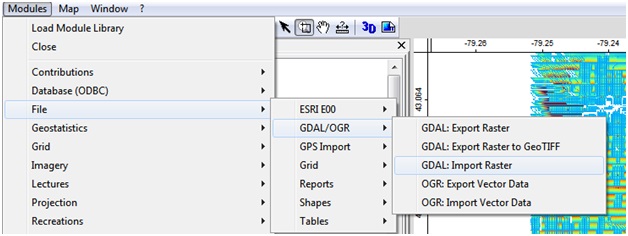
+ | Once you have SAGA up and running by clicking the icon, we must bring in the DEM we created in the steps prior. To do so go to the modules tab, and follow the "File -> GDAL/OGR -> GDAL: Import Raster" command tree, as in the picture below: |
<center>[[Image:bot7.jpg]]</center> |
<center>[[Image:bot7.jpg]]</center> |
||
| + | |||
| + | In the window that is brought up, click the load button to bring up a screen where you can navigate to the location of your DEM. Once the location of the DEM has been entered, click okay. |
||
| + | |||
<center>[[Image:bot8.jpg]]</center> |
<center>[[Image:bot8.jpg]]</center> |
||
<center>[[Image:bot9.jpg]]</center> |
<center>[[Image:bot9.jpg]]</center> |
||
| Line 43: | Line 46: | ||
<center>[[Image:bot11.jpg]]</center> |
<center>[[Image:bot11.jpg]]</center> |
||
<center>[[Image:bot12.jpg]]</center> |
<center>[[Image:bot12.jpg]]</center> |
||
| − | |||
==Conclusions== |
==Conclusions== |
||
Revision as of 13:59, 22 December 2013
Contents
Purpose
The purpose of this wiki is to introduce users to the cross functionality of open source software. It is intended to show how a user can take raw elevation data and create a usable GIS product within a short time period, as to realize geographic phenomena in real world situations such as a spill mitigation scenario.
Introduction
The direction of this project is to show how free and open source software for geospatial applications (FOSS4G) can be implemented as an alternative and in some cases an enhancement to licensed products such as IDRISI and ESRI's ArcMap. To portray this both qGIS and SAGA GIS will be used. The purpose for using two programs is due to ease of use. Where qGIS allows for easy operations to be performed in a somewhat familiar GUI, it does not account for more in depth applications such as flow direction of liquids and the distance they must travel before entering a major tributary. Thus, this tutorial aims to show how to take vector elevation data and transform it to a raster surface which is conducive to modelling and extrapolation.
Software Download and Data Gathering
To download the necessary programs for the purpose of this tutorial, click the following link for the qGIS download portal[1], as well as this link for SAGA GIS's download portal[2]. Upon downloading and installing the correct version as it corresponds to your computer, the next step is to find suitable data for analyzing the area of study. Among many sources, elevation data for Canadian areas can be found easily through such outlets as GeoBase at the following link [3] or GeoGratis at this link [4].
Methods
The project can be divided into two steps: performing the surface interpolation in qGIS and using that produced DEM to determine the overland flow distance in SAGA GIS.
Surface Interpolation in qGIS
The first step is to get qGIS running. Click on the Q emblem placed on your desktop, and upon loading press skip to close the tips menu. Having acquired the data, the elevation points should be brought into qGIS via the add delimited text layer tool found under the “layer” tab on the taskbar.
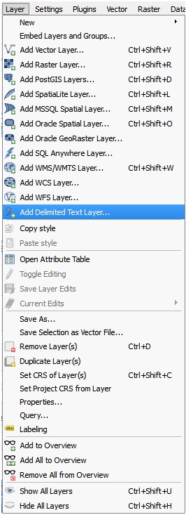
Once you are in the add delimited text layer, simply name the layer as you see fit and toggle on the specifications of the input data table so that it displays properly at the bottom of the screen, as in the following picture:
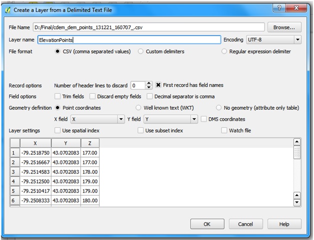
You will now have a block of points the size of your study area. In order to make these points into an interpolated surface we must use the "interpolation" tool under the raster tab, as follows
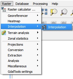
Once in the interpolation window, we find a series of options. Set the interpolation value to that of the elevation value of your dataset, in this case it is column z. If you aren't sure which column is the elevation values, look up the table in excel or open the meta data which came with your elevation points to determine which column it is. For the purposes of hydology, an IDW interpolation is best so we select it as such. Cell size is perhaps the most important attribute to select: set it too big and the resultant map will be complex and take quite a qhile to process, set it too small and you will see generalization and a lack of interpretation abilities. You should try starting small and moving towards big to determine the optimal size. The window should look something like the following:
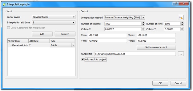
Determine where you would like to save the image and click okay when you are satisfied with the parameters you have selected and you will see this window:
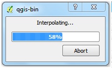
Once processing has finished, dependent on the size of your data set this could take a few minutes or multiple hours, you will see an interpolated surface automatically appear on your map, such as the following:
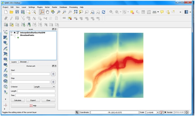
Voila! We have created an interpolated surface. Now we move to SAGA GIS to perform a more in depth analysis.
Determining Overland Flow Distance in SAGA GIS
Once you have SAGA up and running by clicking the icon, we must bring in the DEM we created in the steps prior. To do so go to the modules tab, and follow the "File -> GDAL/OGR -> GDAL: Import Raster" command tree, as in the picture below:
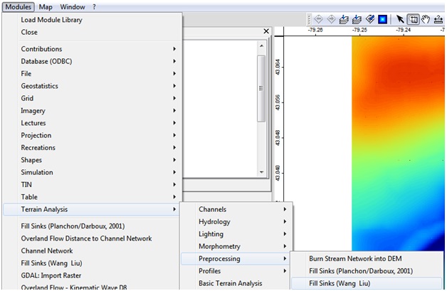
In the window that is brought up, click the load button to bring up a screen where you can navigate to the location of your DEM. Once the location of the DEM has been entered, click okay.
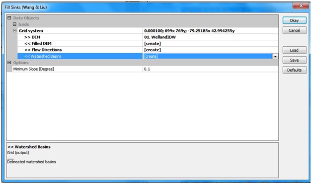
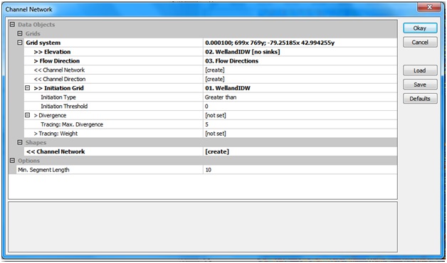
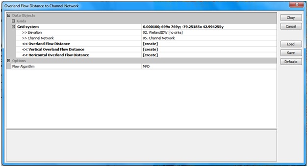
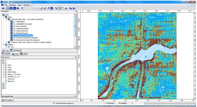
Conclusions
Due to the relatively low accuracy of the data provided, the results can be interpreted visually from the example provided but not quantitatively. However, this tutorial can be recreated with high resolution LiDAR data given the appropriate time and financial allowances to achieve a much more accurate, analyzable result. The purpose of this wiki was to introduce the user to the interoperability between the two programs and the possibilities each program holds.