Introduction to Vegetation Burn Mapping using Open Data Cube

Introduction to Open Data Cube

In this tutorial the main software framework used is called Open Data Cube (ODC), and who’s primary function is to make geospatial data management and performing analysis with large amounts of satellite data easier. It offers a complete system for ingesting, managing, and analyzing a wide variety of gridded data through a combination of many python libraries and a PostgreSQL database. It is extremely flexible in that it offers several cloud and local deployment options, can work with multispectral imagery to elevation models and interpolated surfaces and a multitude of ways to interface with the software. This tutorial will be using Jupyter Notebooks to work with ODC, but a web GUI is also available. A great way to think about ODC is like your own personal, open-source Google Earth Engine. However, unlike Google Earth Engine you are in control over the geospatial data and code you create. If you would like to learn more about the ODC framework you can check out the official website here.

Installation Instructions

At first the installation and configuration process for ODC can appear daunting and complex with several dependencies and a long configuration procedure. It is possible to use ODC on Windows, Linux, or Max, however I find it has the most support and is easiest on Ubuntu. To greatly simplify the installation process ODC has created something called “Cube in a Box”. This is an easy-to-use Docker image that will provide us with a pre-configured reference installation of ODC. Docker uses containerization to package software into units that can be run on most computing environments. More information about Docker and containers can be found here.

Installing Docker

The first step in the installation process will be to install docker. This tutorial is designed for Ubuntu 20.04 but will likely work on other Linux versions.

To install docker run the following command in a new terminal window:

sudo apt-get install docker-compose

And select yes to install any dependencies.

Downloading ODC and Helper Scripts

In this section the Open Data Cube "Cube in a Box" docker configuration will be downloaded from GitHub. Feel free to use the "wget" or "git clone" commands to simplify this process if you undertand how.

Go to: https://github.com/opendatacube/cube-in-a-box and download the all the code using the "Download ZIP" button shown in figure one.

• 

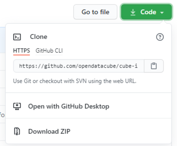
  Figure 1: Download button for Github files.

Unzip these files to a desired location in Ubuntu. I chose the downloads folder. This tutorial takes advantage of a number of helper scripts and a code example from Digital Earth Africa.

Go to: https://github.com/digitalearthafrica/deafrica-sandbox-notebooks And using the previous download instructions grab the all the code.

Next, move the Scripts folder inside the previous cube-in-a-box Notebooks folder. For me I placed Scripts inside /home/admind/Downloads/cube-in-a-box-master/notebooks. Then place the Burnt_area_mapping.ipynb file from the Real_world_examples folder inside deafrica-sandbox-notebooks to the same location as before. This would be /home/admind/Downloads/cube-in-a-box-master/notebooks for me.

The last file is called stac_api_to_dc.py and can be found at: https://raw.githubusercontent.com/opendatacube/odc-tools/develop/apps/dc_tools/odc/apps/dc_tools/stac_api_to_dc.py Place this file inside the Scripts folder you just moved. For me this is now /home/admind/Downloads/cube-in-a-box-master/notebooks/Scripts.

At the end your "cube-in-a-box-master/notebooks" folder should look like figure two.

• 

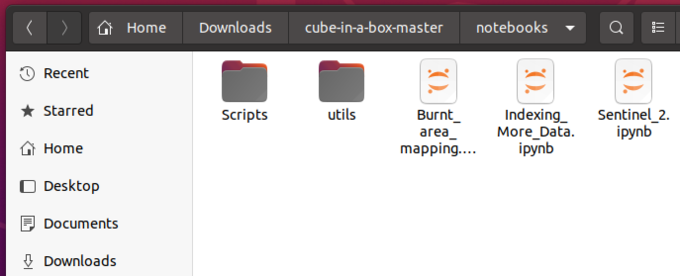
  Figure 2: Final location of moved folders and files.

And have 13 python files in the Scripts folder and the 3 .ipynb files in the Notebooks folder.

Configuring Cube in a Box

The last step of the installation process is to open terminal from the cube-in-a-box-master folder.

This can be done by right clicking anywhere in the cube-in-a-box-master folder and selecting open in terminal.

After this has been done enter the following command into the terminal window: sudo docker-compose up Then after that has completed leave that window open to run and open another terminal with the above process so two terminal windows are open.

In this new terminal enter: sudo docker-compose exec jupyter datacube -v system init Then: sudo docker-compose exec jupyter datacube product add https://raw.githubusercontent.com/digitalearthafrica/config/master/products/esa_s2_l2a.yaml And finally to make sure it works try: sudo docker-compose exec jupyter bash -c "stac-to-dc --bbox='25,20,35,30' --collections='sentinel-s2-l2a-cogs' --datetime='2020-01-01/2020-03-31' s2_l2a"

If everything has ran without error messages in the first terminal window with Docker running open an internet browser and go to "localhost".

That is it! You are now ready to move on to the analysis section.

Performing Vegetation Burn Mapping

As stated previously this tutorial uses a code example from Digital Earth Africa that we have already downloaded and installed.

After following the previous instructions you should see Jupyter Notebooks open in the internet browser window.

Importing Geospatial Data

To import the geospatial data for the region that we will be performing analysis on we run the index script.

Open the file named Indexing_More_Data.ipynb in Jupyter Notebooks. Change the fourth line in the first code cell to appear how it does in figure three.

• 

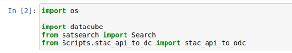
  Lines to be changed in first code box.

Next, we will define the location of interest and the time frame. A box is created around the location with the buffer. This can be extended by increasing the buffer value.

Change the second code cell to appear as follows in figure four:

• 

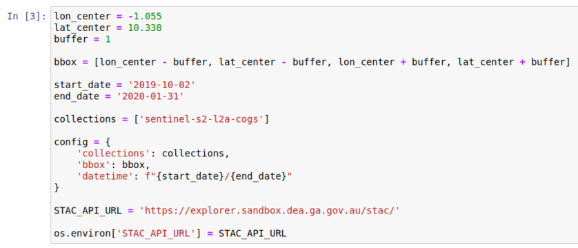
  Figure 4: Entering the location and time frame information.

After this run all the cells in order. It should state that approximately 400 items have been indexed.

Performing Analysis

H

Potential Errors

• If you receive an error during package installation like “Hash Sum Mismatch” then make sure you are using the latest version of Oracle VirtualBox. Version 6.1.16 fixes this bug.
• Ambiguous docker errors including “Cannot Connect to daemon” can be resolved by inserting “sudo” infront of the command you are trying to run.
• If you encounter the following error in figure nine when running scripts in Jupyter Notebooks then you must confirm the entire installation process has been followed.

• 

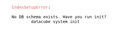
  Figure 9. Database Initialization Error.

Sources and Additional Resources

PASTE HERE