Difference between revisions of "Landscape Change Assessment using Unsupervised Image Classification in GRASS GIS"
| Line 214: | Line 214: | ||
| + | In this section, we will find different ways to view the different layers in our mapset. Data visualization is extremely important for presenting data in ways that help the viewer understand what they are looking at, which allows for better interpretation of results. First, we will use the <u>d.rgb</u> module to view the full images in the “Map Display” window, and then we will use the <u>g.gui.mapswipe</u> (MapSwipe) module to view two layers at the same time. More information about the <u>d.rgb</u> module can be found [https://grass.osgeo.org/grass78/manuals/d.rgb.html here]. More information about the the <u>g.gui.mapswipe</u> (MapSwipe) module can be found [https://grass.osgeo.org/grass78/manuals/g.gui.mapswipe.html here]. |
||
| + | |||
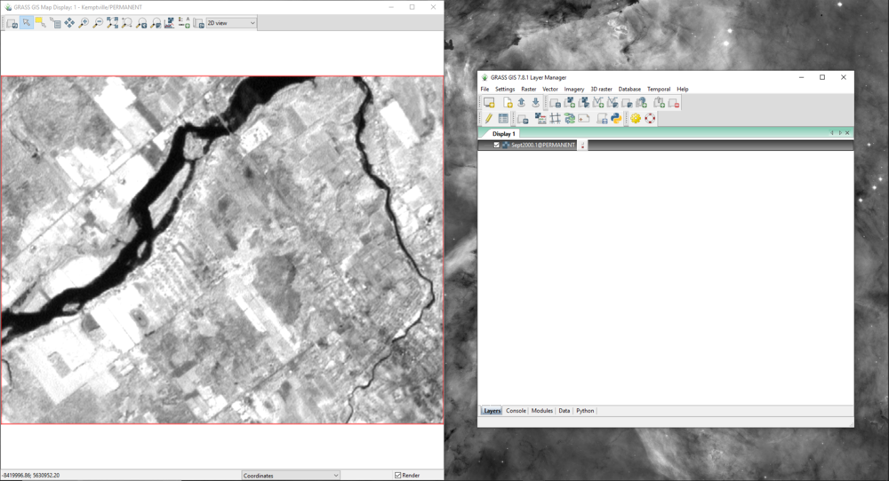
| + | :1) To view a layer in the “Map Display” window, double-click on the layer of interest on the “Data” tab on the “Layer Manager” window. The layer will appear on the “Layers” tab on the “Layer Manager” window and the image will appear on the “Map Display” window (Figure 18). |
||
| + | |||
[[File:LT_DoubleClickLayers_1.png|1000px]] |
[[File:LT_DoubleClickLayers_1.png|1000px]] |
||
| Line 220: | Line 224: | ||
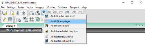
| + | :1) Navigate to the <u> d.rgb </u> module by following the path in Figure 19. |
||
| − | d.rgb [https://grass.osgeo.org/grass78/manuals/d.rgb.html] |
||
| − | :1) |
||
[[File:LT_RGB_1.png|500px]] |
[[File:LT_RGB_1.png|500px]] |
||
| Line 228: | Line 231: | ||
''Figure 19: The path to add an RGB map layer using the d.rgb module.'' |
''Figure 19: The path to add an RGB map layer using the d.rgb module.'' |
||
| + | |||
| − | :1) |
||
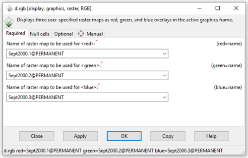
| + | :2) The <u> d.rgb </u> module will open. Because the data being used in this part of the tutorial contains spectral information from bands 2, 3, and 4 (instead of 1, 2, and 3) we will enter the bands in 1, 2, 3 order based on the name they received after importing them. This is because the near-infrared band (4) is identified as the red band (1) by the <u>d.rgb</u> module, and the red band (3) and green band (2) are being identified as the green (2) and blue (3) bands, respectively. This shift is reflected in our input of each of the layers in this module in Figure 20. |
||
| + | |||
[[File:LT_RGB_2.png|500px]] |
[[File:LT_RGB_2.png|500px]] |
||
| Line 234: | Line 239: | ||
''Figure 20: The "d.rbg Module" window showing the required input raster information.'' |
''Figure 20: The "d.rbg Module" window showing the required input raster information.'' |
||
| + | |||
| − | :1) |
||
| + | :3) Click '''Apply''', then '''OK'''. You may now close this module window. The RGB layer will appear in the “Layer Manager” window and in the “Map Display” window as it does in Figure 21. If your image looks different than the one in Figure 21, it is possible that the spectral bands may have been imported in a different order. In this case, just re-arrange the order of the bands in the <u>d.rgb</u> module window and re-apply the change until your bands are ordered correctly and the output image looks like the one in Figure 21. |
||
| + | |||
[[File:LT_RGB_3.png|1000px]] |
[[File:LT_RGB_3.png|1000px]] |
||
| Line 240: | Line 247: | ||
''Figure 21: The RGB map layer output in the "Map Display" window and the selected RGB map layer in the "Layer Manager" window.'' |
''Figure 21: The RGB map layer output in the "Map Display" window and the selected RGB map layer in the "Layer Manager" window.'' |
||
| + | |||
| − | :1) |
||
| + | :4) Now we will use the <u>g.gui.mapswipe</u> (MapSwipe) module to look at two layers simultaneously. Navigate to the <u>MapSwipe</u> module by clicking on '''File > Map Swipe''' (Figure 22). |
||
| + | |||
[[File:LT_MapSwipe_1.png|600px]] |
[[File:LT_MapSwipe_1.png|600px]] |
||
| Line 246: | Line 255: | ||
''Figure 22: The path to use GRASS Map Swipe with the g.gui.mapswipe module.'' |
''Figure 22: The path to use GRASS Map Swipe with the g.gui.mapswipe module.'' |
||
| + | |||
| − | :1) |
||
| + | :5) The <u>MapSwipe</u> module window will open, with another window open on top, the “Select Raster Maps” window (Figure 23). Notice that there is an option to switch to advanced mode, this mode can be seen in Figure 24. Advanced mode gives the user more options for viewing different types of layers. Notice that we could follow the steps above and compare two RGB maps. |
||
| + | |||
[[File:LT_MapSwipe_2.png|500px]] |
[[File:LT_MapSwipe_2.png|500px]] |
||
| Line 254: | Line 265: | ||
[[File:LT_MapSwipe_5.png|400px]] |
[[File:LT_MapSwipe_5.png|400px]] |
||
| − | ''Figure 24: Advanced mode of the "Select Raster Maps" window showing many different options for selecting layers to compare using the g.gui.mapswipe module.'' |
+ | ''Figure 24: Advanced mode of the "Select Raster Maps" window showing many different options for selecting layers to compare using the <u>g.gui.mapswipe</u> module.'' |
| + | |||
| + | |||
| + | :6) Switch back to simple mode and select two layers to compare to one another as I have in figure 25. Click '''OK'''. |
||
| − | :1) |
||
[[File:LT_MapSwipe_3.png|300px]] |
[[File:LT_MapSwipe_3.png|300px]] |
||
| Line 262: | Line 275: | ||
''Figure 25: The completed "Select Raster Maps" window.'' |
''Figure 25: The completed "Select Raster Maps" window.'' |
||
| + | |||
| − | :1) |
||
| + | :7) The “Select Raster Maps” window will close, and you will be able to actively compare the two layers you selected. Click and drag the blue slide at the bottom of the image to see how the two images differ from one another. |
||
| + | |||
[[File:LT_MapSwipe_4.png|500px]] |
[[File:LT_MapSwipe_4.png|500px]] |
||
| Line 268: | Line 283: | ||
''Figure 26: The "Map Swipe" window with displaying band 1 of the September 2000 image on the left, and band 1 of the September 2017 image on the right.'' |
''Figure 26: The "Map Swipe" window with displaying band 1 of the September 2000 image on the left, and band 1 of the September 2017 image on the right.'' |
||
| − | :1) |
||
| + | :8) After you are done experimenting with this tool, close the <u>MapSwipe</u> module window to return to the rest of the tutorial. |
||
| Line 333: | Line 348: | ||
''Figure 35: The "Create Imagery Groups" window showing the creation of a subgroup using the i.group module.'' |
''Figure 35: The "Create Imagery Groups" window showing the creation of a subgroup using the i.group module.'' |
||
| − | === |
+ | ===Category Clustering=== |
i.cluster (Generates spectral signatures for land cover types in an image (the subgroup containing all 3 bands we used above) using a clustering algorithm - this is creates the input for the maxlik tool) |
i.cluster (Generates spectral signatures for land cover types in an image (the subgroup containing all 3 bands we used above) using a clustering algorithm - this is creates the input for the maxlik tool) |
||
Revision as of 21:08, 17 December 2019
Contents
- 1 Purpose
- 2 Introduction to GRASS GIS
- 3 Software Download and Installation
- 4 Data Set
- 5 Methods
- 5.1 Starting GRASS GIS
- 5.2 Adding Extensions
- 5.3 Importing Rasters
- 5.4 Visualizing Layers
- 5.5 Raster Smoothing and Discontinuity Maps
- 5.6 Image Grouping
- 5.7 Category Clustering
- 5.8 Unsupervised Classification
- 5.9 Landscape Change Assessment
- 5.10 Editing the Landscape Change Maps for Distribution
- 5.11 Not Covered in this Tutorial
- 5.12 Additional Resources
- 6 Conclusion
- 7 References
Purpose
The purpose of this tutorial is:
Introduction to GRASS GIS
Software Download and Installation
In this tutorial, GRASS GIS version 7.8.1 for Windows is being used, however this software is also available for Mac and Linux users. The latest version of GRASS GIS may be downloaded here. This website contains very useful information and documentation for users that have never been exposed to GRASS GIS before now. I highly suggest looking at this documentation, as well as this tutorial which provides more information on GRASS GIS.
Data Set
Because this tutorial is being written to demonstrate the ability of GRASS GIS to assess changes in landscapes, a data set has been provided for the user. There are many sources where one can find satellite imagery data, however a data set is being provided to the user so they may follow along with this tutorial without having their own data set. This data set consists of two GeoTiff files acquired using the Earth Observing System (EOS) Landviewer tool. These GeoTiff files contains an image obtained by Landsat 7 on September 7, 2000 and an image obtained by Landsat 8 on September 23, 2017. Both images contain imagery of the same area of interest (AOI) which consists of a 40.04 km² square area centered at 45.03001°N 75.68135°W. This area is located in Kemptville, Ontario, an area which has undergone development since the early 2000s to accommodate for increased population sizes. The population of Kemptville is expected to rise given it's close proximity to Ottawa, making it an ideal location for commuters to reside, which means that further development is also expected.
To download the imagery required for this tutorial, click on the links in the table below. This will begin downloading each of the files to your computer.
| Landscape Change Assessment Data Set | |
|---|---|
| Data Information | Data File |
| GeoTIFF file for raster imagery from September 7, 2000 with bands 2, 3, and 4 (Landsat 7) | September 2000 File |
| GeoTIFF file for raster imagery from September 23, 2017 with bands 2, 3, and 4 (Landsat 8) | September 2017 File |
| GeoTIFF file for raster imagery from September 7, 2000 with bands 1, 2, and 3 (Landsat 7) | [September 2000 Visible Bands File] |
| GeoTIFF file for raster imagery from September 23, 2017 with bands 1, 2, and 3 (Landsat 8) | [September 2017 Visible Bands File] |
Methods
Starting GRASS GIS
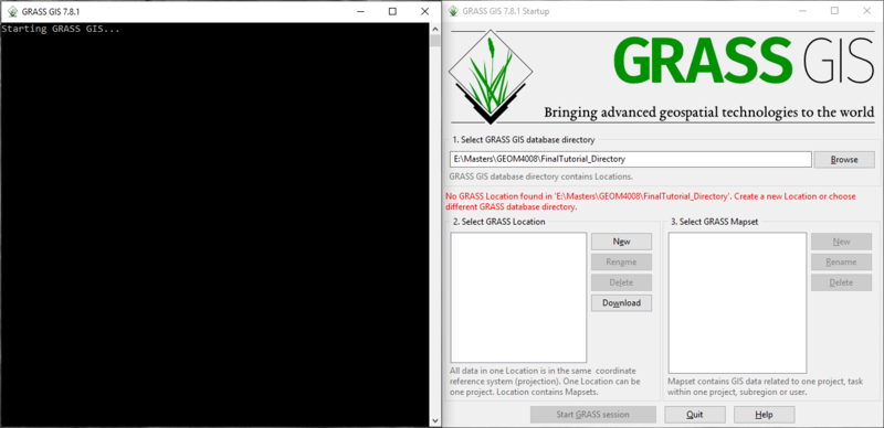
Once GRASS GIS is properly installed on your computer, you may locate it and open the program. The GRASS GIS startup interface is where the user will set their database directory and define characteristics of the project location (Figure 1). To begin using GRASS, we must first set a working (database) directory, with a project location and a mapset. The data directory is a folder on your computer where you will store all of the data for your project. The project location is a subdirectory within the database directory that contain spatial information about the project you are working on. This spatial information includes things like the coordinate system and the projection information. Within a project location, you may have multiple mapsets which contain different layers and maps that are all related to one another based on the characteristics of the project location. In this tutorial, we will use the “PERMANENT” mapset which is created automatically within the project location. More information about starting with GRASS for the first time can be found in the Quickstart Guide here.
Figure 1: The GRASS GIS Startup Interface
- 1) Click Browse under “Select GRASS GIS database directory” to navigate to the folder you wish you use as the database directory on your computer. The message seen in red font in Figure 1 should appear.
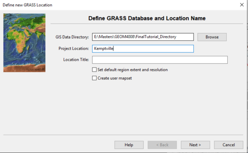
- 2) Click New under “Select GRASS Location” to create a new project location. The window seen in Figure 2 should appear.
Figure 2: The "Define New GRASS Location" window where the user selects a Data Directory and Project Location.
- 3) Choose a name for your project location and type it into the appropriate box. In this example, the name of the project location is “Kemptville”. It is best to keep the project location name simple, and if desired, a location title can be input which describes the project location in more detail.
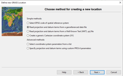
- 4) Click Next and Figure 3 should appear. In this example, we will use the second method (“Read projection and datum terms from a georeferenced data file”) to create our new project location.
Figure 3: The "Define New GRASS Location" window where the user chooses a method for creating a new Location.
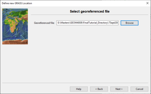
- 5) Click Next to select a georeferenced file (Figure 4).
Figure 4: The "Define New GRASS Location" window where the user selects a georeferenced file.
- 6) Click Browse and navigate to the GeoTIFF file you downloaded earlier called “7Sept2000.tiff”.
- 7) Click Next to review your selection and the projection definition on the Summary window (Figure 5.)
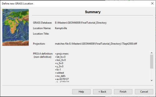
Figure 5: The "Define New GRASS Location" window summary page.
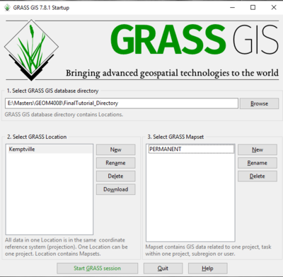
- 8) Click Finish to create the project location. The Startup window should now appear as it does in Figure 6.
***You may receive a pop-up at this stage that asks you if you want to import the 7Sept2000.tiff file into your newly created location. Click Yes.***
Figure 6: The "GRASS Startup" window with a Directory, Location, and Mapset selected.
- 9) Click Start GRASS session in green font at the bottom, left of the startup interface. Three windows should appear:
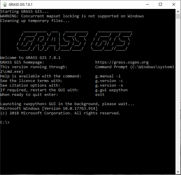
- The “GRASS Command” window (Figure 7). You may use this window to call on different modules (tools) or you can find them using the graphical user interface (GUI).
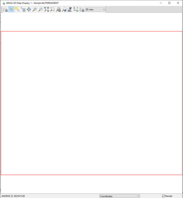
- The “GRASS Map Display” window (Figure 8). This is where our different map layers will appear when they are selected.
- The “GRASS Layer Manager” window (Figure 9). This is the main GUI where we will be working in this tutorial. Take notice of the different tabs along the bottom of the window (Layers, Console, Modules, Data, Python). The “Layers” tab is where the different map layers will appear when they are selected or created. The next important tab is the “Modules” tab where you can find all the modules (tools) we will use in this tutorial. The last tab we will use in this tutorial is the “Data” tab, which shows you all of the project locations and mapsets that are stored in the current database directory.
Figure 7: The "GRASS Command" window.
Figure 8: The "GRASS Map Display" window.
Figure 9: The "GRASS Layer Manager" window.
Adding Extensions
Because GRASS is open-source software, users are free to create their own extensions. These extensions are also called “add-ons”, and are modules created by users to carry out specific tasks that are not offered by any of the default modules. More information about extensions, including manual pages for all of the extensions and information about developing an add-on can be found here.
There are two extensions that we will download in this tutorial. This first extension is the r.smooth.seg extension which will be used to smooth and segment our images based on spectral data, and the second is r.change.info which is used to compare classified images to one another to determine locations of change.
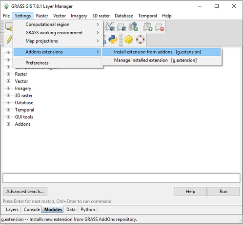
- 1) Navigate to the g.extension module by clicking on Settings > Addons Extensions > Install Extension from Addons (Figure 10).
Figure 10: The path to install new add-ons in GRASS GIS.
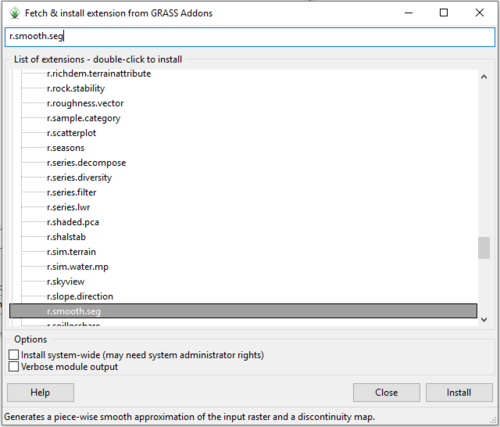
- 2) Type r.smooth.seg into the search bar at the top of the g.extension window (Figure 11).
Figure 11: The "Fetch & Install Extension from GRASS Add-ons" window with search results for the r.smooth.seg add-on.
- 3) Click on the r.smooth.seg module in the list of extensions. Notice that there is a description of what the module does in the bottom of the window.
- 4) Double-click on the extension or select it and click Install in the bottom right corner of the window to install the extension.
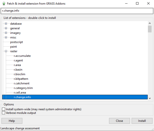
- 5) Now we will install the second extension we need by typing "r.change.info" into the search bar at the top of the g.extension window (Figure 12).
Figure 12: The "Fetch & Install Extension from GRASS Add-ons" window with search results for the r.change.info add-on.
- 6) Double-click on the extension to install it.
- 7) At this point, GRASS GIS must be restarted to load the new extensions.
- 8) Upon opening GRASS GIS for the second time, navigate to the “Modules” tab at the bottom of the "Layer Manager" window.
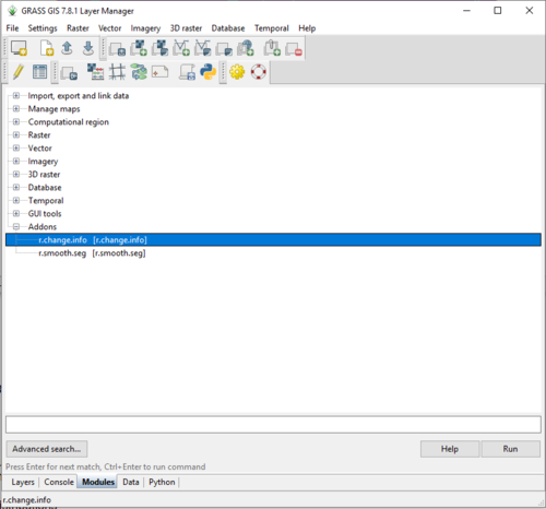
- 9) Click the + sign beside the “Addons” category to expand it (Figure 13).
- 10) To run modules through the “Modules” tab, double-click on them, or select it and click Run in the bottom right corner.
Figure 13: The "Layer Manager" window with the Modules tab open, and the newly installed add-on selected.
Importing Rasters
Now that all of the modules we need are loaded into GRASS, we can import our data. To do this, we will use the r.in.gdal module. This module imports raster data into GRASS using the GDAL library, which supports many different file formats. More information about this module can be found here. More information about the GDAL library can be found here.
Because we used the 7Sept2000.tiff file as the georeferenced file for our projection location, this file should already be imported. This can be confirmed on the “Data” tab on the “Layer Manager” window.
For the remainder of this tutorial, I will be using the 7Sept2000.tiff raster as an example in each of the steps. However, the steps in the remainder of the tutorial (apart from the Landscape Change Assessment section) will need to be carried out twice: once for our September 2000 data, and once for our September 2017 data.
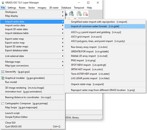
- 1) Navigate to the r.in.gdal module by clicking on File > Import Raster Data > Import of Common Raster Formats (Figure 14).
Figure 14: The path to import raster data using the r.in.gdal module.
- 2) The r.in.gdal module window will open. Notice the tabs along the top of the window, which each have different options that you can apply to your raster. The “Command Output” tab is very useful because it shows you the progress of the module and provides you with information about the module outputs. This tab shows up in all of the module windows and will be referred to in later steps.
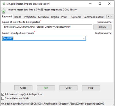
- 3) Fill in the input and output information on the “Required” tab. The input here is the location of the imagery you downloaded at the beginning of the tutorial (in this case the 7Sept2000.tiff image). The output is the name you would like the raster to have (Figure 15).
- 4) Once you have this information filled out, click the green Run button to run the module.
Figure 15: The "r.in.gdal Module" window showing input and output raster information on the "Required" tab.
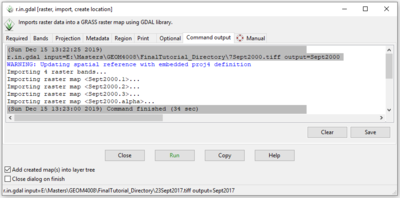
- 5) Click on the “Command Output” during/after the run to watch the progress and see information about the module output (Figure 16).
Figure 16: The "r.in.gdal Module" window showing the "Command Output" tab.
- 6) After the module is complete, repeat these steps for the 23Sept2017.tiff imagery.
- 7) Close the r.in.gdal module window and navigate to the “Data” tab on the “Layer Manager” window.
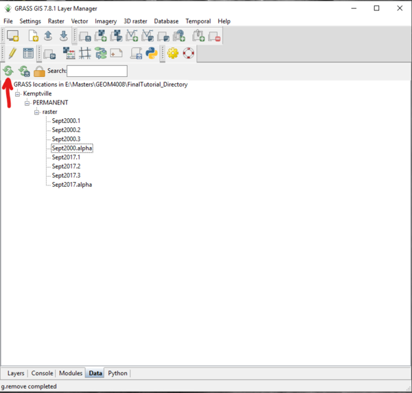
- 8) Confirm that the imagery you have just imported appears here. If the layers are not present, press the green “Refresh” button and they will appear (Figure 17). Notice that there are 4 layers imported for each image you imported. This is because GRASS separates the 3 spectral bands (2, 3, 4) imported from the image and also includes an alpha channel (Sept2000.alpha) that contains NULL cells.
Figure 17: The "Refresh" button on the "Data" tab in the "Layer Manager" window.
Visualizing Layers
In this section, we will find different ways to view the different layers in our mapset. Data visualization is extremely important for presenting data in ways that help the viewer understand what they are looking at, which allows for better interpretation of results. First, we will use the d.rgb module to view the full images in the “Map Display” window, and then we will use the g.gui.mapswipe (MapSwipe) module to view two layers at the same time. More information about the d.rgb module can be found here. More information about the the g.gui.mapswipe (MapSwipe) module can be found here.
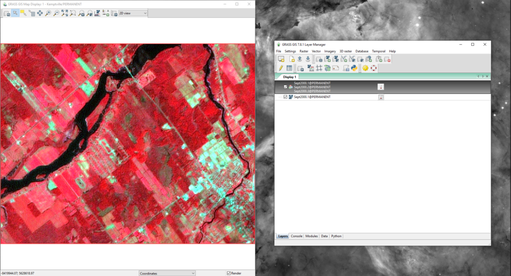
- 1) To view a layer in the “Map Display” window, double-click on the layer of interest on the “Data” tab on the “Layer Manager” window. The layer will appear on the “Layers” tab on the “Layer Manager” window and the image will appear on the “Map Display” window (Figure 18).
Figure 18: The "Map Display" window and "Layer Manager" window showing the "Sept2000.1" layer.
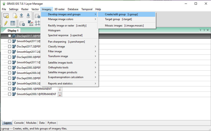
- 1) Navigate to the d.rgb module by following the path in Figure 19.
Figure 19: The path to add an RGB map layer using the d.rgb module.
- 2) The d.rgb module will open. Because the data being used in this part of the tutorial contains spectral information from bands 2, 3, and 4 (instead of 1, 2, and 3) we will enter the bands in 1, 2, 3 order based on the name they received after importing them. This is because the near-infrared band (4) is identified as the red band (1) by the d.rgb module, and the red band (3) and green band (2) are being identified as the green (2) and blue (3) bands, respectively. This shift is reflected in our input of each of the layers in this module in Figure 20.
Figure 20: The "d.rbg Module" window showing the required input raster information.
- 3) Click Apply, then OK. You may now close this module window. The RGB layer will appear in the “Layer Manager” window and in the “Map Display” window as it does in Figure 21. If your image looks different than the one in Figure 21, it is possible that the spectral bands may have been imported in a different order. In this case, just re-arrange the order of the bands in the d.rgb module window and re-apply the change until your bands are ordered correctly and the output image looks like the one in Figure 21.
Figure 21: The RGB map layer output in the "Map Display" window and the selected RGB map layer in the "Layer Manager" window.
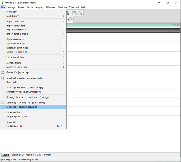
- 4) Now we will use the g.gui.mapswipe (MapSwipe) module to look at two layers simultaneously. Navigate to the MapSwipe module by clicking on File > Map Swipe (Figure 22).
Figure 22: The path to use GRASS Map Swipe with the g.gui.mapswipe module.
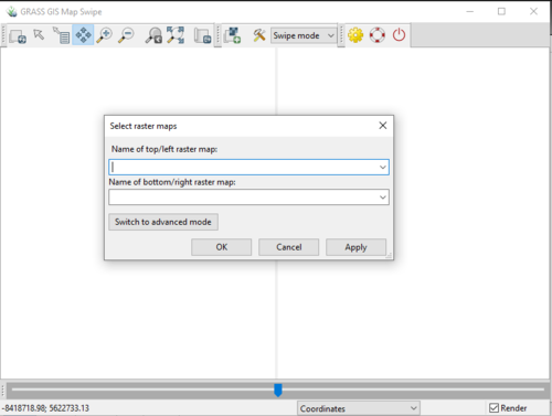
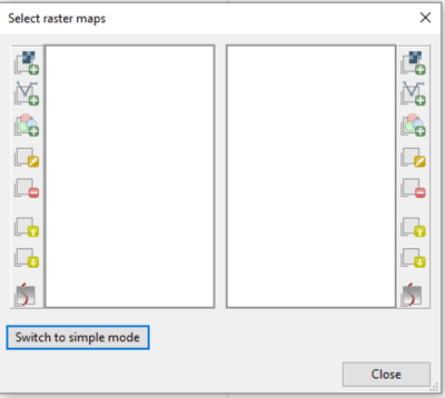
- 5) The MapSwipe module window will open, with another window open on top, the “Select Raster Maps” window (Figure 23). Notice that there is an option to switch to advanced mode, this mode can be seen in Figure 24. Advanced mode gives the user more options for viewing different types of layers. Notice that we could follow the steps above and compare two RGB maps.
Figure 23: The "Select Raster Maps" window from the Map Swipe module.
Figure 24: Advanced mode of the "Select Raster Maps" window showing many different options for selecting layers to compare using the g.gui.mapswipe module.
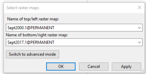
- 6) Switch back to simple mode and select two layers to compare to one another as I have in figure 25. Click OK.
Figure 25: The completed "Select Raster Maps" window.
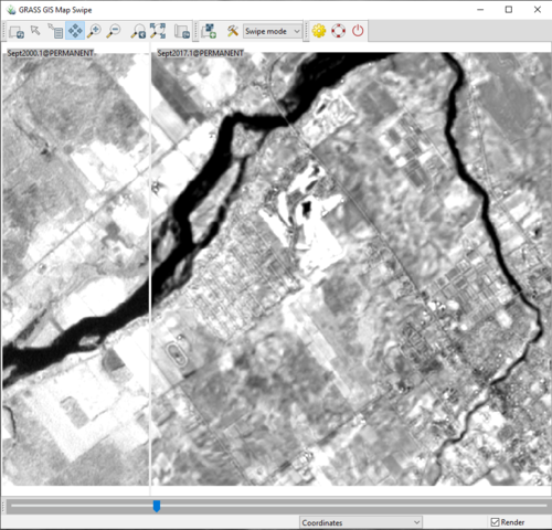
- 7) The “Select Raster Maps” window will close, and you will be able to actively compare the two layers you selected. Click and drag the blue slide at the bottom of the image to see how the two images differ from one another.
Figure 26: The "Map Swipe" window with displaying band 1 of the September 2000 image on the left, and band 1 of the September 2017 image on the right.
- 8) After you are done experimenting with this tool, close the MapSwipe module window to return to the rest of the tutorial.
Raster Smoothing and Discontinuity Maps
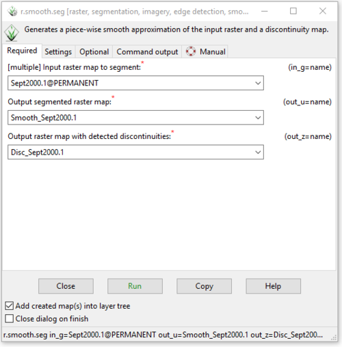
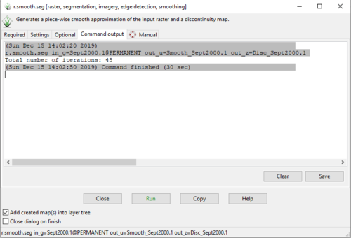
r.smooth.seg - image pre-processing (takes place before segmentation - smooths out each band individually - also identify segments from each individual band)
- 1)
Figure 27: The "r.smooth.seg Module" window with the completed input and output information on the "Required" tab.
- 1)
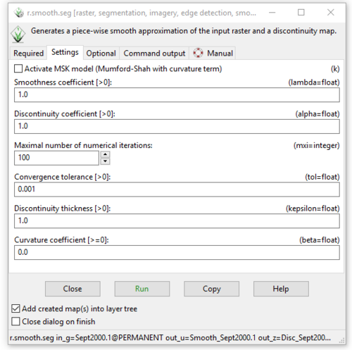
Figure 28: The "Settings" tab in the "r.smooth.seg Module" window showing the different variables that can be adjusted.
- 1)
Figure 29: The "Command Output" tab in the "r.smooth.seg Module" window showing the output information.
- 1)
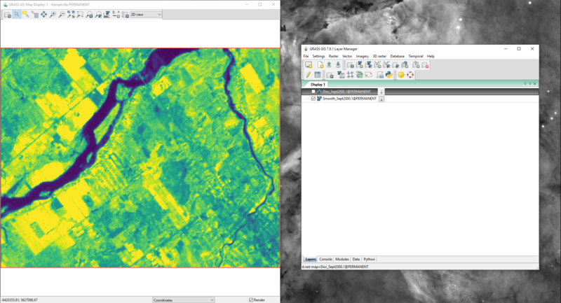
Figure 30: The "Map Display" window with the smoothed map output for band 1 of the September 2000 data using the r.seg.smooth module.
- 1)
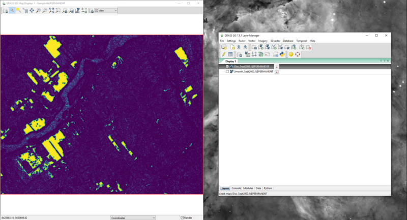
Figure 31: The "Map Display" window with the discontinuity map output for band 1 of the September 2000 data using the r.seg.smooth module.
Image Grouping
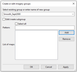
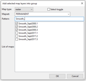
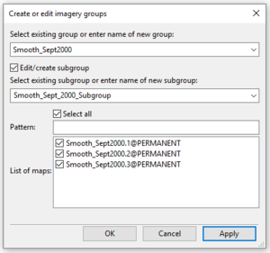
i.group - group bands 2, 3, 4 together, and create a subgroup containing all 3 of the images (sub-groups required for the cluster step - group and subgroup contain the same (all 3) images)
- 1)
Figure 32: The path to the i.group module in the "Layer Manager" window.
- 1)
Figure 33: The "Create or Edit Imagery Groups" window from the i.group module.
- 1)
Figure 34: The "Add Selected Layers into Group" window from the i.group module.
- 1)
Figure 35: The "Create Imagery Groups" window showing the creation of a subgroup using the i.group module.
Category Clustering
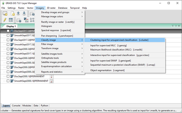
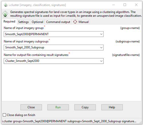
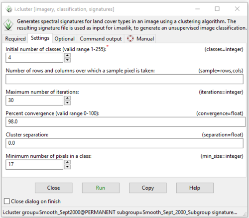
i.cluster (Generates spectral signatures for land cover types in an image (the subgroup containing all 3 bands we used above) using a clustering algorithm - this is creates the input for the maxlik tool)
- 1)
Figure 36: The path to the i.cluster module in the "Layer Manager" window.
- 1)
Figure 37: The "i.cluster Module" window showing the input and output information on the Required tab
- 1)
Figure 38: The "i.cluster Module" window showing the variables available on the Settings tab.
Unsupervised Classification
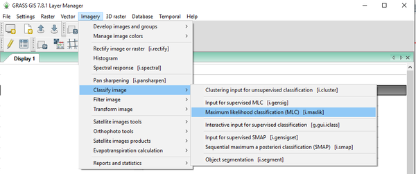
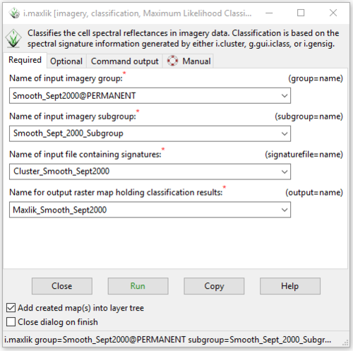
i.maxlik
- 1)
Figure 39: The path to the i.maxlik module in the "Layer Manager" window.
- 1)
Figure 40: The "i.maxlik Module" window showing the input and output information on the Required tab
- 1)
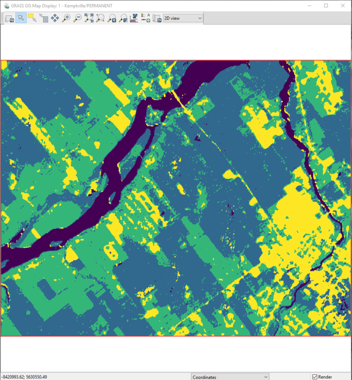
Figure 41: The classified map output for September 2000 created by the i.maxlik module.
- 1)
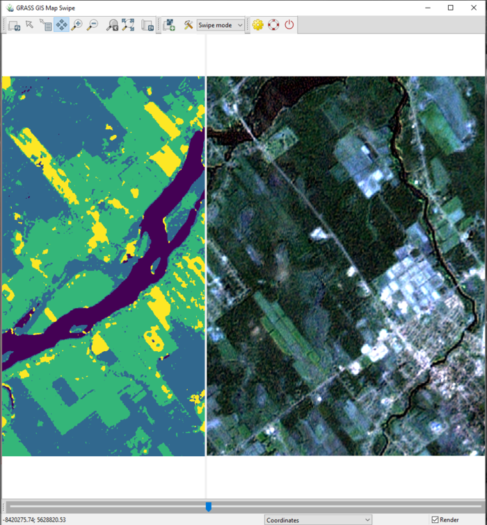
Figure 42: The Map Swipe window showing the classified imagery for September 2000 on the left, and the original imagery for bands 1, 2, and 3 for September 2000 on the right.
Landscape Change Assessment
r.change.info
- 1)
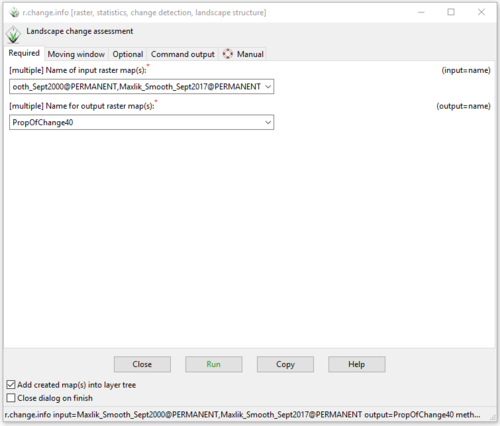
Figure 43: The "r.change.info Module" window with the input and output information on the Required tab for the "PropOfChange40" layer.
- 1)
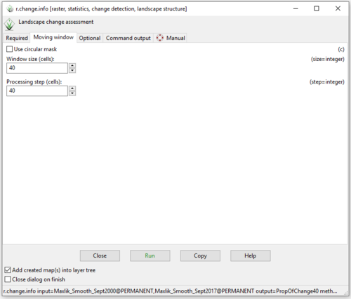
Figure 44: The "r.change.info Module" window with variable information on the "Moving Window" tab, where step = 40 cells.
- 1)
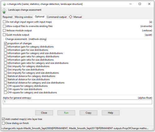
Figure 45: The "r.change.info Module" window with the "proportion of changes" change assessment selected on the "Optional" tab.
- 1)
Figure 46: The output from the r.change.info module with the "PropOfChange40" layer in the "Map Display" window.
- 1)
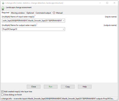
Figure 47: The "r.change.info Module" window with the input and output information on the "Required" tab for the "PropOfChange10" layer.
- 1)
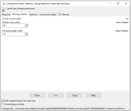
Figure 48: The "r.change.info Module" window with variable information on the "Moving Window" tab, where step = 10 cells.
- 1)
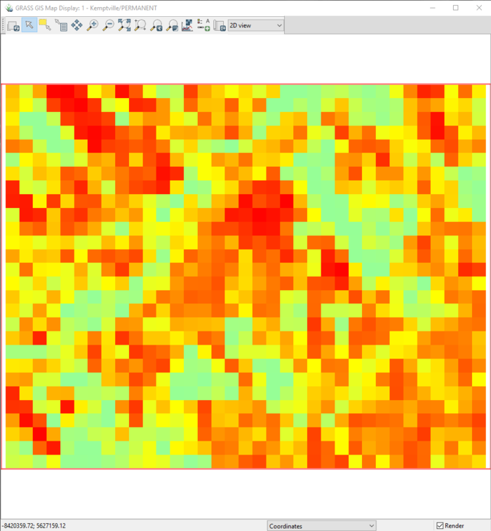
Figure 49: The output from the r.change.info module with the "PropOfChange40" layer in the "Map Display" window.
- 1)
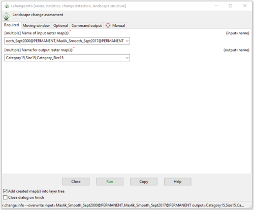
Figure 50: The "r.change.info Module window" with the input and output information on the "Required" tab for the "Category15","Size15", and "Category_Size15" layers.
- 1)
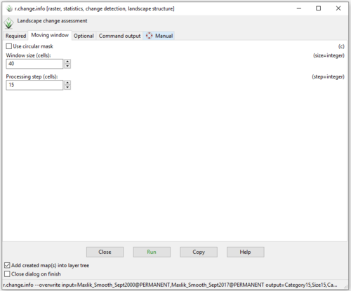
Figure 51: The "r.change.info Module" window with variable information on the "Moving Window" tab, where step = 15 cells..
- 1)
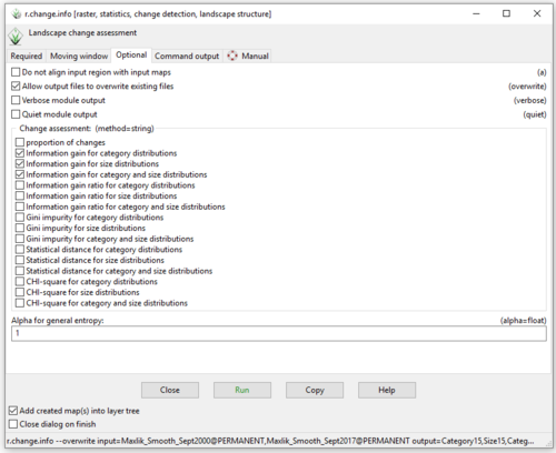
Figure 52: The "r.change.info Module" window with "Information Gain for Category Distributions", "Information Gain for Size Distributions", and "Information Gain for Category and Size Distributions" change assessments selected on the Optional tab.
- 1)
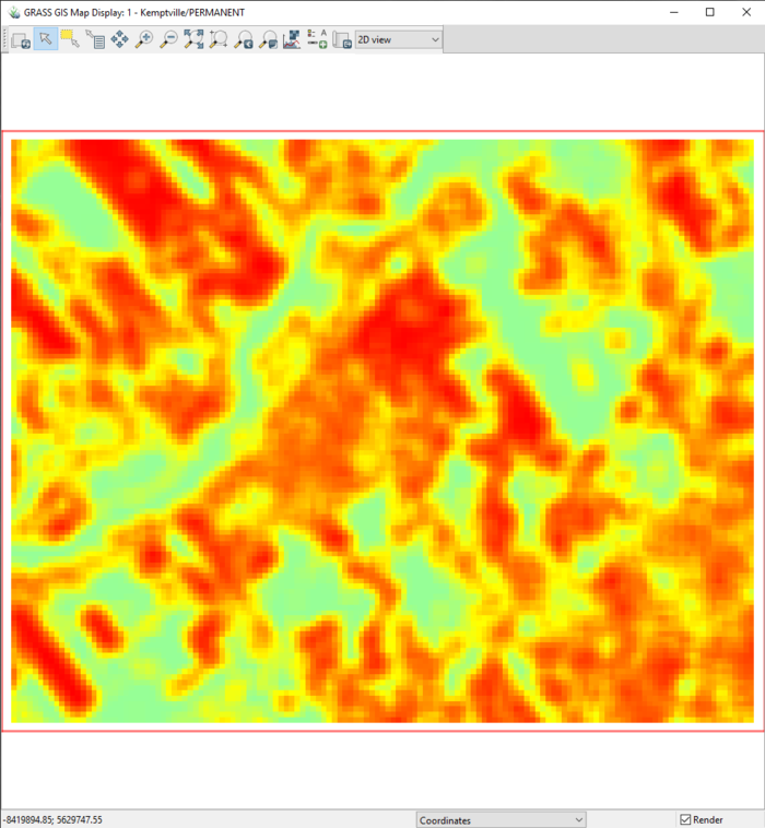
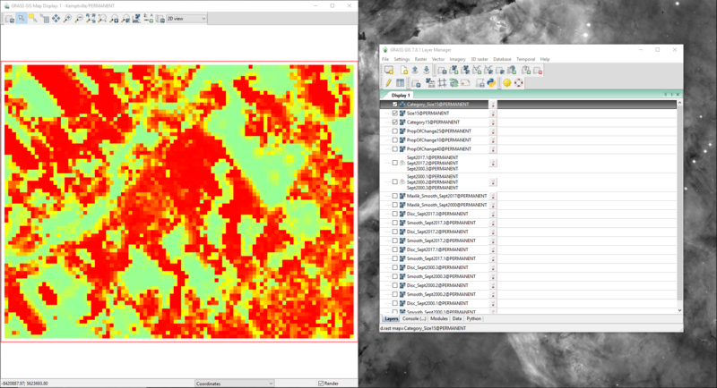
Figure 53: The output from the r.change.info module with the "Category_Size15" layer in the "Map Display" window.
- 1)
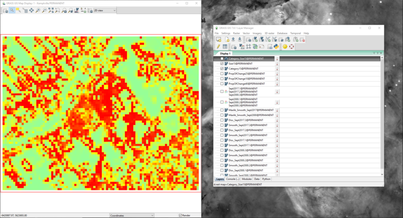
Figure 54: The output from the r.change.info module with the "Size15" layer in the "Map Display" window.
- 1)
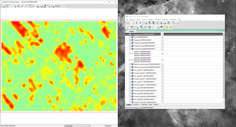
Figure 55: The output from the r.change.info module with the "Category15" layer in the "Map Display" window.
Editing the Landscape Change Maps for Distribution
- 1)
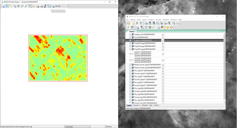
Figure 56: The "Category15" layer in the "Map Display" window zoomed out.
- 1)
Figure 57: The path to the "Add Raster Legend" module (d.legend) in the "Map Display" window.
- 1)
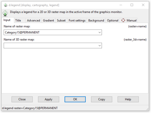
Figure 58: The "Input" tab in the "d.legend Module" window.
- 1)
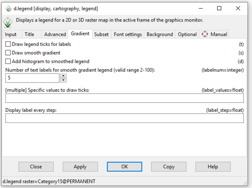
Figure 59: The "Gradient" tab in the "d.legend Module" window showing where the labels for the gradient legend may be altered.
- 1)
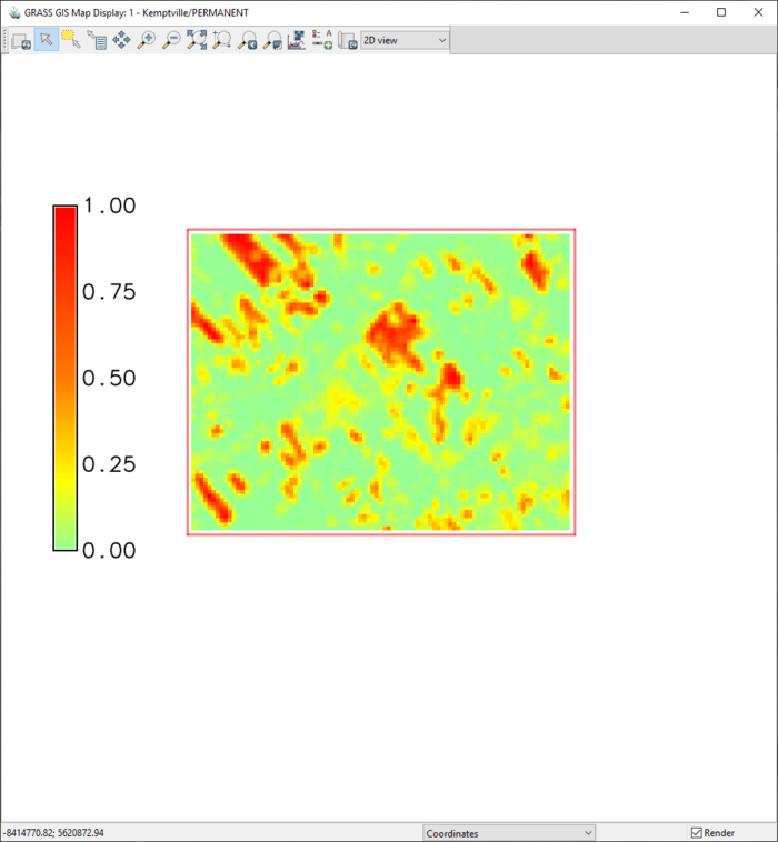
Figure 60: The "Category15" layer with a gradient legend.
Not Covered in this Tutorial
Additional Resources
Conclusion
References
https://renx.ca/kemptville-building-boom-retail-residential/
Earth Observing System (EOS) Landviewer [1]
GRASS GIS Software [2]
