Modelling Air Mass Time Over Water with Hysplit, SAGA GIS, and Python

Introduction

In this tutorial, we will explore how to combine a vector line with raster surface information to extract quantitative information about the conditions underneath the line. There are numerous possible applications for this: we can look at an air mass moving over different land cover types, the impact of pollutants on river currents, or the habitats an animal prefers to travel through. Here, we will focus on one particular application, that of how long an air mass spends over water. However, the techniques can be applied to many different problems.

For our purposes, the line will represent the trajectory of an air mass, with each segment representing a certain amount of time. We are interested in how long the air mass spent over water. This is of interest since air masses that spend a long time over water tend to have higher humidity which can affect how much evaporation occurs at further points.

Given a raster grid that determines whether a cell is water or not, we can evaluate this by the following general process:

Split the line into segments based on the raster grid
Determine whether or not the segment is over water and how much time it represents
Sum the length of time represented by segments that are over water.

Here, I will briefly demonstrate how to use a National Oceanic and Atmospheric Administration (NOAA) tool called Hysplit to determine the backtrajectory of an air mass from a point in time and space over a week. I will then show how Python can be used to extract that data and, using SAGA GIS, calculate the amount of time spent over water for the trajectory. The process can be adapted with minimal changes to use other trajectories and raster data.

Prerequisites

Thorough comfort with Python and command line tools would be greatly beneficial. You might find [tutorial on SAGA and Python] useful to start learning with. Comfort with your operating system is recommended. The optional Hysplit component requires some comfort with FTP servers. This tutorial is focused on the Windows environment, but all the software described should also work in a Unix environment with suitable modifications.

Setup

Demonstration Files

You can download these demonstration files which contain the code and some sample files to run it with.

Hysplit

I have provided an example Hysplit data file in the demonstration files if you’d rather not follow these steps. However, if you are interested in air mass trajectory analysis, you may find these useful.

Visit https://www.ready.noaa.gov/HYSPLIT_util.php and install the Tcl/Tk graphical user interface and the Ghostscript / Ghostview postscript viewer. Make sure you install Ghostscript and GSview to their default directories to avoid complications.
You can then download and install Hysplit https://www.ready.noaa.gov/HYSPLIT_hytrial.php
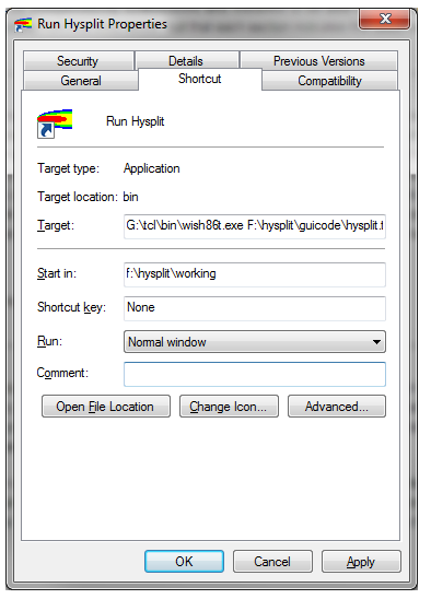
To run Hysplit on Windows, you’ll need to edit the shortcut to tell it to run the Hysplit Tcl code with the Tcl interpreter. Right click on the shortcut to Hysplit on your desktop or start menu and click Properties. Edit the “Target” field to have the path to the Tcl executable called wish86t.exe. On other platforms, you may have to take similar steps.
You can then test that you can launch Hysplit.

SAGA GIS

SAGA GIS can be installed from this link: https://sourceforge.net/projects/saga-gis/

Python

Python can be installed from this link: https://www.python.org/downloads/

Data

Air Mass Modelling

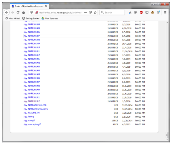
To use Hysplit, you will need information on atmospheric conditions to successfully generate a backtrajectory. Some example data is included in Hysplit. If you’d like to run your own analysis, you can download monthly data from NOAA’s ARL FTP server ftp://arlftp.arlhq.noaa.gov/pub/archives/narr/. This can be done with most web browsers or an FTP client. The files are named NARRYYYYMM, so for our tutorial let’s download the December 2019 file (NARR201912).

Surface Raster Data

There are a number of sources that can be used for surface water data. Here, we’ll use the General Bathymetric Chart of the Oceans (GEBCO) gridded bathymetric data. It provides depths or elevations throughout the world and is completely open to the public. https://www.gebco.net/data_and_products/historical_data_sets/

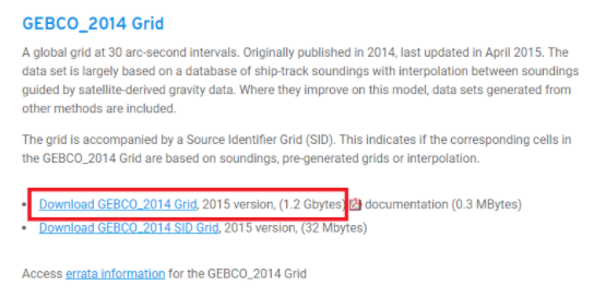
Download the GEBCO 2014 grid (or use the updated 2020 grid if you’d like but it is much larger). It will come as a NetCDF file, one of our first tasks will be to convert it to a format suitable for SAGA GIS.

Working Directory

Hysplit works best under the installation directory. If you won’t be using Hysplit, you can put your files anywhere. Otherwise, create a folder under your Hysplit working directory called “tutorial”. Put your NARR file in that directory.

Tutorial

Hysplit Back Trajectory Modelling (Optional)

If you’re not interested in air mass trajectory modelling, you can skip this step and download my sample “tdump” file. Save it to your working folder, then just read through the instructions so you have some sense of what the file contains. Launch Hysplit and click on “Menu”. We’re going to run a backtrajectory of the air mass over Carleton University at 2 m height on the last day of exams (Dec 21, 2019 at 9PM) for one week. Carleton University is located at 45.3876 N by 75.6960 W.

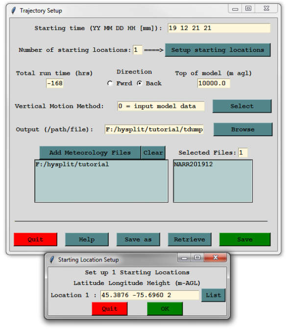
Open the Trajectory menu and select “Setup Run”. Set the parameters as follows, leave the other parameters the same

Starting Time: 19 12 21 21
Number of starting locations 1
Total run time: -168
Direction: Back
Output path: A file called “tdump” in your working directory
Clear the existing meteorology files and add the NARR file you downloaded earlier.
Click the “Setup starting locations” button and enter the latitude, longitude (remember west is negative!), and starting height. Click OK, then click Save.

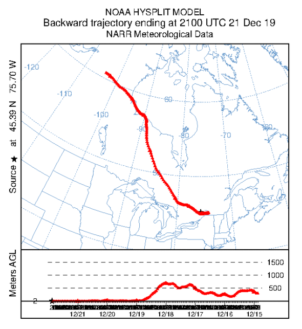
Select “Run Model” from the Trajectory model. You should see a dialog window appear and the model run. When you see “Complete Hysplit” appear, you can click the Exit button. You can see the trajectory by clicking on the Trajectory menu, the Display submenu, and then the Trajectory option. Keep all the defaults and click “Execute Display”. If you have Ghostscript / GSView set up right, you should see a map of North America and a red line indicating where the air mass travelled in the week before reaching Carleton University. The graph below shows the height of the air mass over land as it travelled.

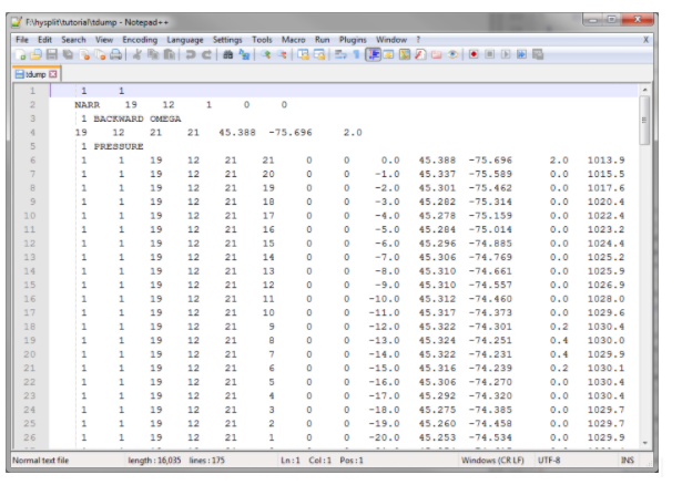
At this point, you should have a “tdump” file in your working directory. Open it up and let’s look at the contents. The first few lines tell us a bit about how the run was configured - you can see the start time, the coordinates, the input files, etc. Starting on the sixth line is the output data in space-delimited format. The columns are as follows:

Trajectory number
Grid number
Year
Month
Day
Hour
Minute
Forecast hours
Time since start time (in hours)
Latitude
Longitude
Height above ground
Pressure

We’ll work more with this data in a few sections. Right now, let’s get our GEBCO grid ready for use.

Converting GEBCO 2014 NetCDF to SAGA GIS Grid Format

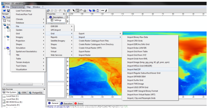
Launch SAGA GIS. While we’ll be using the command line interface for the most part, we will convert the NetCDF file using the graphical interface. Open the “Import NetCDF” tool by going to the Geoprocessing menu, then to File, Grid, Import, and finally Import NetCDF. For “File”, select the .nc file you downloaded and unzipped. Check “Save to File” and select your working directory for the Save to Path. Click Ok and let it run. When it finishes, you should have a set of files including a “.sdat” file. Make a note of the path to the .sdat file, you’ll need it later. You can then close SAGA.

File:File:Et2020 saga detailed example.png

Air Mass Time Over Water

To determine the time the air mass has spent over water, we will need to take several steps in both Python and with SAGA GIS. To simplify the workflow, we’ll use the Python subprocess module to call SAGA’s command line interface from within Python. The steps we will need to take are as follows:

Extract the trajectory from the tdump file
Segment the trajectory into sections based on the GEBCO grid
Extract the grid value for each section. Negative values are water, positive values are land.
Using the grid values, calculate a total time over water for the trajectory

Create a new Python file called watertime.py in your working directory.

Extracting the trajectory

To extract the trajectory, we will read the trump file into a Python list of points. Each point will be a dictionary object with all the information about that point on the trajectory, but notably including the x and y coordinates. The Python code for this follows. Note that we skip a few lines at the beginning that correspond to data that isn’t part of the trajectory.

import subprocess
# LineSegment class is stored in lineseg.py
from lineseg import LineSegment

# Location of your tdump file
tdump_file = r"F:\hysplit\tutorial\tdump"

# Store the points in this object
points = []

# Open the file for reading
print("Reading trajectory information")
with open(tdump_file, "r") as handle:
    # split the file into lines
    lines = handle.read().split("\n")
    # Track the number of files
    trajectory_file_count = None
    # Track the number of starting points
    starting_point_count = None
    # Flag to skip the output type line
    skip_output_type = True
    # loop through lines
    for line in lines:
        # Split the line based on spaces and remove empty ones
        data = list(filter(lambda x: not x == "", line.split(" ")))

        # Skip blank lines
        if len(data) == 0:
            continue
        
        # The first line we encounter is the trajectory file count
        if trajectory_file_count is None:
            trajectory_file_count = int(data[0])
            continue
        # Then we skip lines equal to the trajectory file count
        if trajectory_file_count > 0:
            trajectory_file_count -= 1
            continue
            
        # Repeat for trajectory points
        if starting_point_count is None:
            starting_point_count = int(data[0])
            continue
            
        if starting_point_count > 0:
            starting_point_count -= 1
            continue
        
        # Skip the output flag line if not already done
        if skip_output_type:
            skip_output_type = False
            continue
        
        # Now we can read points from the trajectory
        points.append({
            "start_point": int(data[0]),
            "grid": int(data[1]),
            "year": int(data[2]),
            "month": int(data[3]),
            "day": int(data[4]),
            "hour": int(data[5]),
            "minute": int(data[6]),
            "forecast": int(data[7]),
            "timestep": float(data[8]),
            "y": float(data[9]),
            "x": float(data[10]),
            "z": float(data[11]),
            "p": float(data[12]),
        })
print("{} points found".format(len(points)))

If your trajectory is in another format, you can adapt this method as long as the latitude, longitude, and timestep are present.

Segment the trajectory

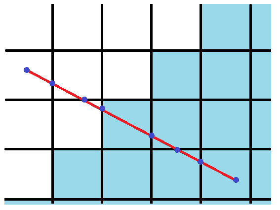
Given a grid aligned to the x- and y-axis, we can segment a straight line to pieces that extend over a single grid cell by splitting the line where it intersects either the horizontal or vertical lines of the grid. The illustration below demonstrates this by cutting the line at the blue dots.

To do this in Python is fairly straight-forward. Here, I’ve provided a class that accomplishes the task. It takes two points for the start and end of a segment and then splits it into smaller segments based on a grid with a specific origin and spacing between the horizontal and vertical lines in the grid.

(python 2)

We can then loop through the segments and split each one into a set of subsegments which correspond to the grid cells. The GEBCO 2014 grid is centered on 0 N by 0 W and has half arc-minute grid sizes. We’ll also calculate the time over that particular subsegment and put in a blank classification for now. Note that we convert the measurements from degrees to arc minutes just to make the math easier later since we have a half arc minute grid.

(python 3)

Extracting grid values using SAGA

SAGA has a tool which will add a column to a point class with the value of a raster grid underneath the point. We’ll leverage this tool and our line segments to extract the grid values for our segments. First, we’ll build a list of points that have to be extracted. We’ll make it a unique set of grid centerpoints to reduce the number of points we need to process.

(python 4)

Next, we’ll need to call a few SAGA commands from the command line. The three steps we’ll need from SAGA are

Convert the CSV file into a points class (with shapes_points)
Extract the grid values onto the points (with shapes_grid)
Convert the points class back to something readable (with io_shapes)

To do this, we will use the subprocess module which lets us call an executable file from within Python. Here’s the first step, which creates the points class from the CSV file. Note that we tell it where it can find the SAGA executable and the CSV file, as well as the name of a new point shape file to make and that the longitude is in the first column (#0) and the latitude is in the second column (#1). We then pass the command over to the subprocess module to execute, store the output in variables, and wait for it to finish. If there was an error, we’ll exit our script at this point and you can debug your command. You should replace the file paths to the appropriate ones for your installation of SAGA and to your working folder.

(python 5)

We’ll run the next two processes in a similar fashion, to extract the grid values and then to output it to a tab-seperated value file. Update the file paths as needed to point to your working folder and to your sdat file.

(python 6)

Next, we’ll take the tab-separated value file and convert it to a lookup table. We can use this table with the segments to find out if the values are over water (negative) or not (positive).

(python 7)

Calculating Time Over Water

We’re almost done at this point. Next, we’ll need to classify the segments as land (0) or water (1) and calculate the total time over water for the whole line. Note that we could combine these steps, but they’re broken down into two steps here for clarity and in case you want to do a more complicated analysis that might require all of the segments to be classified first.

(python 8)

Running the Script

When you run it, if you have all the values set correctly, you should get output that looks like the following.

Scaling The Process

This tutorial has outlined how to accomplish this task for a single trajectory file. If you’re interested in scaling up to run many points, there are a few things you can alter for efficiency:

First, build a list of unique grid midpoints using all of your input files and run this through SAGA. The calls to SAGA are one of the slowest parts of this process and you can save time by doing this. Keep this in a TSV file.
Next, you can then go input file by input file, load and segment the trajectory, and perform the lookup. You can then save the output to a CSV file.
Finally, if desired, Hysplit has a command line interface as well. You can perform a series of trajectory calculations using it and tie in the results to the above code to get a fully automated workflow for trajectory and time over water calculations.

Code for this is not fully explained here, but is provided in the demonstration files if it is of interest.