Random Forest Supervised Classification Using Sentinel-2 Data

Introduction to Multi-spectral Imaging

Multispectral imaging (MSI) captures image data within specific wavelengths ranges across electromagnetic spectrum. MSI detects different images through instruments that are sensitive to different wavelengths of light thus allowing for distinction in land-type. MSI is a highly informative form of imaging technique as it can move beyond visible light range and can detect and extract data that the human eye fails to capture. Sentinel 2 is an Earth Observation mission from the Copernicus programme that acquires high resolutions of multispectral imagery by conducting frequent visits over a given area. Sentinel-2 is a polar-orbiting Earth Observation Mission from the Copernicus programme that conducts multispectral high-resolution imaging for land monitoring to provide, for example, imagery of vegetation, soil and water cover, inland waterways, and coastal areas. Sentinel-2 can also deliver information for emergency services. Sentinel-2A was launched on 23 June 2015 and Sentinel-2B followed on 7 March 2017. The Sentinel-2 has 13 bands of multispectral data in the visible, near infrared and short-wave infrared part of the spectrum. This tutorial applies images captured by the Sentinel 2A satellite, which provides similar functions to the ones mentioned above.

Supervised and Random Forest Classification

Supervised Classification is a technique used for extracting information from image data. The process includes classification of pixels of an image into different classes based on features of the pixels. Supervised classification can be conducted in 2 main stages. The first stage is called Training Stage and the latter is called Classification Stage. In the training stage of the process, a set of vectors called training sample is established by the user through which the supervised classification is conducted. The number of classifiers is depended upon the number of inputs by the user. For example, if the user identifies 5 different land cover classes in its training data, the supervised classification conducted will output an image of the scene using the data and will have 5 different class distinctions. This tutorial uses a specific type of supervised classification technique called Random Forests.

Random Forest Classification is a Supervised form of classification and regression. Random forest or random decision forests are a form of Model Ensembling techniques. Model Ensembling attempts to aggregate large number of test models to improve accuracy in classification and regression. Random Forest works on the principle of Model Ensembling and helps provide accurate low-cost classified images using a baseline of training data. Higher the training data for classification, higher the accuracy in the end product.

Software and Data Acquisition

This section provides information on the software's and data to be used to conduct the processes listed in the tutorial.

Sentinel Application Platform (SNAP)

The Sentinel Application Platform - or SNAP - in short is a collection of executable tools and Application Programming Interfaces (APIs) which have been developed to facilitate the utilisation, viewing and processing of a variety of remotely sensed data. The functionality of SNAP is accessed through the Sentinel Toolbox. The purpose of the Sentinel Toolbox is not to duplicate existing commercial packages, but to complement them with functions dedicated to the handling of data products of earth observing satellites.

The following tutorial uses SNAP Version 8.0. The software is open source and can be downloaded through the following link: http://step.esa.int/main/download/snap-download/. Specific toolboxes for data processing of data from different Sentinel Satellites can also be downloaded through the link.

This tutorial uses a Windows 64-bit operating system with Windows 11 and 16GB of RAM. The software can also run on a Mac OS X, Unix 64-bit and Windows 32-Bit. The software recommends having at least 4GB of memory. To run the 3D World Wind View, it is recommended to have a 3D graphics card with updated drivers. However, this tutorial will not be using 3D World Wing View. SNAP will work on 32- and 64-bit Windows, Mac OS X and Linux.

Microsoft Excel / OpenOffice Calc

The tutorial also uses Microsoft Excel Software to Conduct Kappa Coefficient Analysis. The software can be downloaded from the link: https://www.microsoft.com/en-ca/microsoft-365/p/excel/cfq7ttc0k7dx/?activetab=pivot%3aoverviewtab

However, the software is only available through purchase therefore an alternative software to conduct similar processes is Microsoft OpenOffice Calc. This software is free to use and can be downloaded from the link: https://openoffice.en.softonic.com/download

Tutorial and SNAP Data

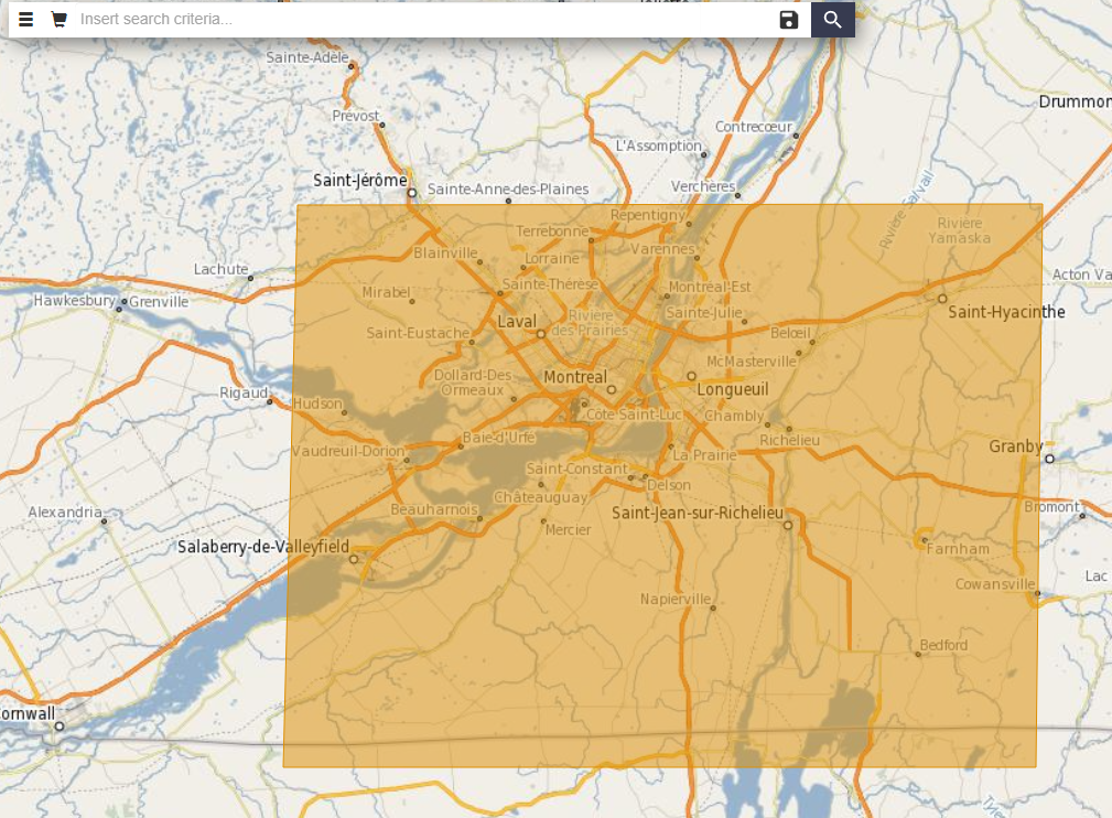
To acquire the data used in the tutorial, you will have to create a free account with Scihub, also known as, Copernicus Open Access Hub. The free to use and open access hub allows access to Sentinel 1, 2, 3, 5P data. Go to the link: https://scihub.copernicus.eu/dhus/#/home and to the top right corner, you will find a symbol of account login. Below that you will find a link to “Sign Up”. Click that and fill out the information. Once your account is set up, you can begin by entering the same link and typing in the search bar, the type of data you wish to download. A different approach through which data can be acquired is by creating a polygon space over the area you desire to use for the tutorial. Hover over the map and zoom In or Out depending on the scale of the area you wish to use. Once you have the extent you wish to use, CLICK Once the Right Pointer on you Mouse. A line will appear, extend the line to your liking, and CLICK the Right Pointer again and now you will have a 2-side completed polygon. Repeat the steps until you have a complete polygon, once that is achieved, DOUBLE CLICK the right button on you Mouse, this will concretize your area of interest. Refer to Figure 1 Below for guidance on how the polygon will look.

Figure 1: Screenshot of the polygon space created over AOI.

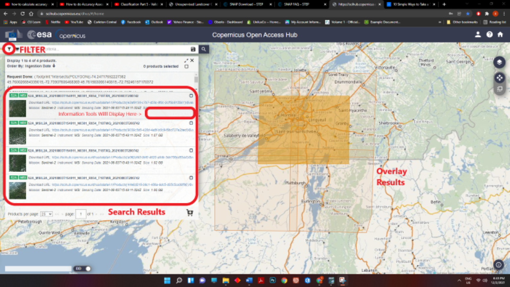
Next, Click the SEARCH button near the search bar. You will now have different polygon overlays of imagery data acquired from different Sentinel Satellites.

Figure 2: Screenshot of the window with search results and filter button navigation.

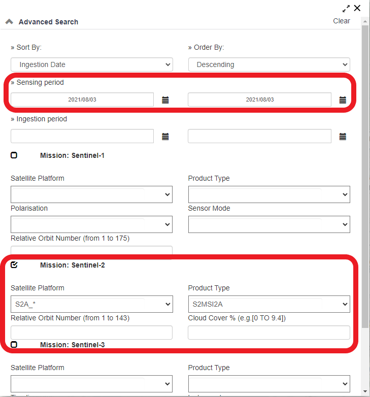
To further narrow you search to specific dates and Satellite Types, Click the FITLER tab and change the settings according to your wishes. The window will look like the Figure 3 below:

Figure 3: Screenshot of the filter window tab.

The data used in this tutorial cab be attained using the following parameters in the filter tab: Location: Montreal Sensing Period: 08/03/2021-08/03/2021 Satellite Type: Sentinel 2A Product Type: MSI2A Dataset Name: S2A_MSIL2A_20210803T154911_N0301_R054_T18TXR_20210803T200742 This can also be found in the Figure 3. Once the filters have been applied. The best overlaying polygon (one that covers all/or most of the area of interest) can then be downloaded through hovering over the result and clicking the DOWNLOAD ARROW SYMBOL on the BOTTOM RIGHT of the Search Result.

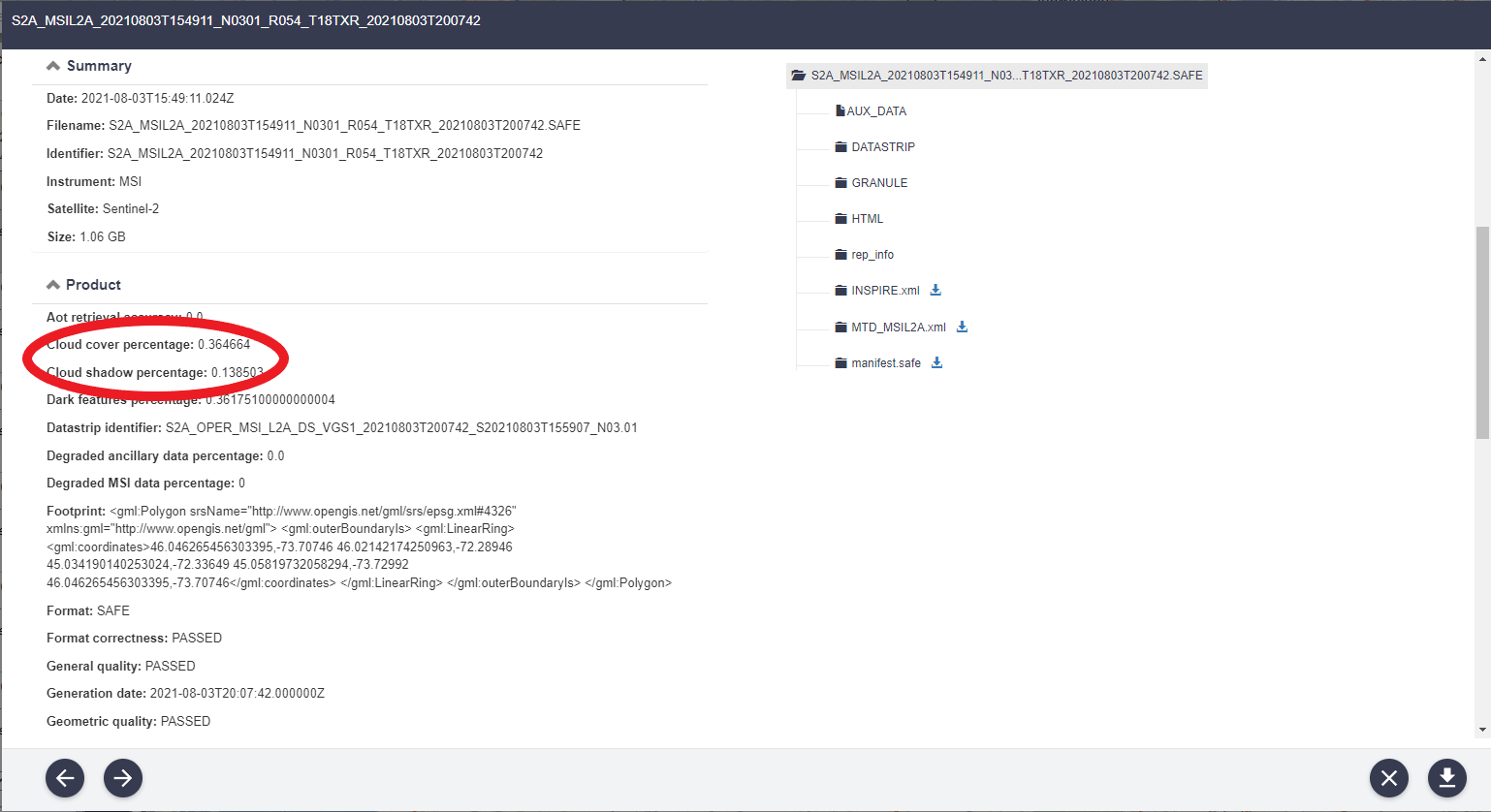
It is important to attain data that has the least amount of cloud cover. This information can be found by clicking the EYE SYMBOL beside the sensing output search. Under PRODUCT INFORMATION, you will find the CLOUD COVER PERCENTAGE. This value should be near 0 as this allows for a more accurate SUPERVISED CLASSIFICATION. An example of this information can be found in the Figure 4 below:

Figure 4: Screenshot of the product details tab, displaying the cloud cover percentage of the acquired image.