Difference between revisions of "Supervised Classifications using Google Earth Engine"
| Line 3: | Line 3: | ||
=Getting Started= |
=Getting Started= |
||
We will now begin preparing the image(s) that we will be classifying. |
We will now begin preparing the image(s) that we will be classifying. |
||
| + | |||
| + | ==Creating Geometry== |
||
==Displaying Images== |
==Displaying Images== |
||
| Line 22: | Line 24: | ||
[[File:GettingStarted.png|750px|thumb|center]] |
[[File:GettingStarted.png|750px|thumb|center]] |
||
| − | We can make it so that the image loads in with a specific combination of bands, but unfortunately, we cannot apply a specific stretch. If you know the range you want to apply, you can add that |
+ | We can make it so that the image loads in with a specific combination of bands, but unfortunately, we cannot apply a specific stretch. If you know the range you want to apply, you can add that. |
<syntaxhighlight lang="javascript">Map.addLayer(image, bands = ['B4', 'B3', 'B2'])</syntaxhighlight> |
<syntaxhighlight lang="javascript">Map.addLayer(image, bands = ['B4', 'B3', 'B2'])</syntaxhighlight> |
||
| Line 28: | Line 30: | ||
This will load the image in with bands 4, 3, and 2, being in the R, G, and B slots. |
This will load the image in with bands 4, 3, and 2, being in the R, G, and B slots. |
||
| − | == |
+ | ==Image Preperation== |
Google Earth Engine has a large selection of remote sensing data to choose from. In this example, I will be using the ' |
Google Earth Engine has a large selection of remote sensing data to choose from. In this example, I will be using the ' |
||
USGS Landsat 8 Collection 1 Tier 1 Raw Scenes' collection. This is a collection of the highest quality images available through Landsat 8. |
USGS Landsat 8 Collection 1 Tier 1 Raw Scenes' collection. This is a collection of the highest quality images available through Landsat 8. |
||
| Line 78: | Line 80: | ||
// Clip to extent |
// Clip to extent |
||
var clipAfter = compAfter.clip(extent);</syntaxhighlight> |
var clipAfter = compAfter.clip(extent);</syntaxhighlight> |
||
| + | |||
| ⚫ | |||
| + | Now that you have the image you would like to use, there is an optional step that will vary based on the application of your classification. By using band math you can create and add a new band into an image. Since my location has been largely impacted by burn, I will create a Normalized Burn Ratio band. Doing this is fairly simple, there is already a normalizedDifference function in Google Earth Engine, so one way of creating it is as such: |
||
| + | |||
| + | <syntaxhighlight lang="javascript"> |
||
| + | // UDF to create and add an NBR band |
||
| + | var calcNBR = function(image){ |
||
| + | var NBR = image.normalizedDifference(['B5', 'B7']).rename("NBR"); // NBR is the normalized difference between NIR and SWIR |
||
| + | var newImage = image.addBands(NBR); |
||
| + | return newImage; |
||
| + | }; |
||
| + | |||
| + | // Add a normalized burn ratio band into the image |
||
| + | var bands = ['B2', 'B3', 'B4', 'B5', 'B6', 'B7', 'NBR']; |
||
| + | var clipAfter = calcNBR(clipAfter).select(bands);</syntaxhighlight> |
||
| + | |||
| + | Notice that before I added the NBR band to 'clipAfter' I created a variable holding all the bands that I want to use in the classification. This is not essential but it will definitely come in handy and removes 'useless' bands such as coastal aerosols and the panchromatic band. |
||
| + | |||
| + | '''NOTE:''' This is not the only way to do this, you can use band math to do calculations within the bands as well. For further examples of this check ______________!!!!!!__!__!__!_ |
||
| + | |||
| + | After creating a cloud-free mosaic of my study area, adding an NBR band, and changing the visual parameters to show SWIR, NIR, and Green, as R, G, and B, respectively (a common colour infrared to identify burn), this is what my image currently looks like: |
||
| + | |||
| + | |||
| + | [[File:BeforeafterCI.png|500px|thumb|center|Left: Image with normal RGB bands. Right: Colour infrared to view burn. ]] |
||
| − | ==Preparing Images== |
||
| ⚫ | |||
=Getting Training Data= |
=Getting Training Data= |
||
| Line 96: | Line 120: | ||
error matrix |
error matrix |
||
==Run on Chosen Image== |
==Run on Chosen Image== |
||
| − | ===Calculating Area of Each Class |
+ | ===Calculating Area of Each Class=== |
===Creating a Chart of Landcover=== |
===Creating a Chart of Landcover=== |
||
Revision as of 10:31, 17 November 2020
Introduction
Getting Started
We will now begin preparing the image(s) that we will be classifying.
Creating Geometry
Displaying Images
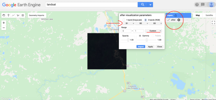
Displaying images in Google Earth can take some getting used to. I am aware that I have not shown you how to create an image yet, bear with me. This step is important and will be repeated throughout the tutorial which is why I want to show you now. The application in itself is fairly simple, it takes one line:
Map.addLayer(image)
It is as simple as that; however, there are likely two issues that you will immediately notice:
- You will notice that the image is dark. This is because it will automatically set the range of pixel values from 0-1. This is typically not enough to represent an image.
- Once this issue is fixed, the colours will look off. This is due to it automatically setting bands 1, 2, and 3 as R, G, and B. These are not the proper bands for the colours.
Remedying these issues is fairly simple, just follow these steps:
- Navigate to the image settings:
- Select the dropdown next to range. I would suggest setting the stretch to either 3σ or 100%. This step only alters the appearance on the map and does not change the image in anyway. Therefore it is largely for personal preference.
- Change the bands to R: B4, G: B3, B: B2. This is the combination for Landsat 8, if you are using any other satellites with different band combinations it may be different.
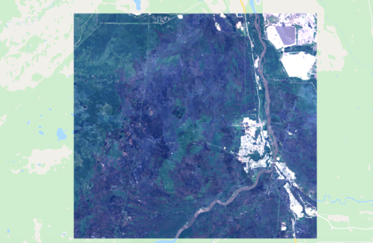
With these changes, your image should look something like this:
We can make it so that the image loads in with a specific combination of bands, but unfortunately, we cannot apply a specific stretch. If you know the range you want to apply, you can add that.
Map.addLayer(image, bands = ['B4', 'B3', 'B2'])
This will load the image in with bands 4, 3, and 2, being in the R, G, and B slots.
Image Preperation
Google Earth Engine has a large selection of remote sensing data to choose from. In this example, I will be using the ' USGS Landsat 8 Collection 1 Tier 1 Raw Scenes' collection. This is a collection of the highest quality images available through Landsat 8.
Define a variable 'L8' so that you can easily reference this entire collection:
var L8 = ee.ImageCollection('LANDSAT/LC08/C01/T1');
Creating a Cloud-Free Mosaic
Now that we have a variable named L8 that is linked to the Landsat 8 collection that we want, we can begin to filter images and choose what we want. For this example, I will create a cloud-free mosaic of Fort McMurray in the month after the major fire that swept through in May of 2016. I have created two functions for this, one that creates a cloud mask and the other that creates a simple composite from a collection of images.
- By utilizing the 'BQA' band present in Landsat 8 imagery, we can create a cloud mask to remove any cloud pixels that may alter the result. I created a function that will select any pixel that has cloud cover with even moderate confidence. The function will return a mask that removes all of these pixels from an image. Note that I have commented on this one fairly heavily due to it be slightly confusing at first.
- I should add again, if you haven't already explored all the bands of your chosen imagery, do. There are plenty of interesting things that can be used.
// Cloud mask for L8 imagery
var L8CloudMask = function(L8) {
  var qa = L8.select('BQA');  //selects the BQA (quality) band
  var CloudOrShadow = qa.bitwiseAnd(1<<4) //chooses pixels where cloud is present
            .and(qa.bitwiseAnd(1<<6)) //and pixels where cloud confidence ic greater than 34%
            .or(qa.bitwiseAnd(1<<8))  //or pixels where cloud shadow confidence is greater than 34%
            .or(qa.bitwiseAnd(1<<12));  //or pixels where cirrus confidence is greater than 34%
  var masked = L8.mask(); //creates a mask
  return L8.updateMask(CloudOrShadow.not()).updateMask(masked); //updates mask to remove any pixels as described above in 'CloudOrShadow'
};
- Now onto the composite. This is a much simpler function, it simply intakes a collection of images and uses the built in 'simpleComposite' function to combine them into the best possible image.
// Function to create composite
var createComp = function(collection) {
  var comp = ee.Algorithms.Landsat.simpleComposite({
    collection: collection,
    asFloat: true
  });
  return comp;
};
- With the two main functions created, we can now use a few lines to create our final image.
// Select all images within June 2016 that touch the extent and have the least removed from the cloud mask
var after = ee.ImageCollection('LANDSAT/LC08/C01/T1')
        .filterDate('2016-06-01', '2016-06-30')
        .filterBounds(extent)
        .map(L8CloudMask);

// Create composite of images chosen above
var compAfter = createComp(after);
// Clip to extent
var clipAfter = compAfter.clip(extent);
Adding Bands
Now that you have the image you would like to use, there is an optional step that will vary based on the application of your classification. By using band math you can create and add a new band into an image. Since my location has been largely impacted by burn, I will create a Normalized Burn Ratio band. Doing this is fairly simple, there is already a normalizedDifference function in Google Earth Engine, so one way of creating it is as such:
// UDF to create and add an NBR band
var calcNBR = function(image){
  var NBR = image.normalizedDifference(['B5', 'B7']).rename("NBR"); // NBR is the normalized difference between NIR and SWIR
  var newImage = image.addBands(NBR);
  return newImage;
};

// Add a normalized burn ratio band into the image
var bands = ['B2', 'B3', 'B4', 'B5', 'B6', 'B7', 'NBR'];
var clipAfter = calcNBR(clipAfter).select(bands);
Notice that before I added the NBR band to 'clipAfter' I created a variable holding all the bands that I want to use in the classification. This is not essential but it will definitely come in handy and removes 'useless' bands such as coastal aerosols and the panchromatic band.
NOTE: This is not the only way to do this, you can use band math to do calculations within the bands as well. For further examples of this check ______________!!!!!!__!__!__!_
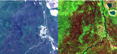
After creating a cloud-free mosaic of my study area, adding an NBR band, and changing the visual parameters to show SWIR, NIR, and Green, as R, G, and B, respectively (a common colour infrared to identify burn), this is what my image currently looks like:
Getting Training Data
Create Landcover Polygons
Gather Data from Polygons
Create Training and Validation Sets
Assess Useability of Data
histograms etc
Classification
Test on Validation Data Set
error matrix


