Beginner's Guide to TINs, DEMs and Contours Using QGIS
Introduction and Intent
There are two purposes of this tutorial, the first being to introduce new Geographic Information Systems (GIS) users to the uses of Triangular Irregular Networks (TINs), Digital Elevation Models (DEMs) and traditional cartographic contour lines. The second objective of this tutorial is to show the processes that users can follow to create, manipulate and use these three datatypes within the QGIS open source software. The three aforementioned datatypes are related in one key way, they are all different means of representing elevation data. They differ in the ways they accomplish this and the types of data they use. These distinctions are discussed in the Vector vs Raster section of this tutorial.
QGIS
QGIS is an open source, free Geographic Information System that lets users display and modify geometric datasets. This means that data that incorporates any sort of geographic positioning, such as incorporating coordinate points into a spread sheet, can be used to create data that exists in a 2 dimensional space. This is a very powerful tool for any user that wants to communicate spatial information to a client, peer or superior. Skills in the use of GISs like QGIS increase the user’s ability to disseminate information easily and are in demand in fields ranging from transport, mineral exploration and exploitation, construction and far more.
Downloading QGIS
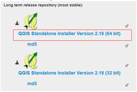
For the purposes of this tutorial, you will have to download a copy of QGIS from the download portal here (https://qgis.org/en/site/forusers/download.html). There will be three versions of QGIS that are accessible here, each with a 32 and 64 bit version. The version we want is “QGIS Standalone Installer Version 2.18 (64 bit)” as seen in Figure 1.
Once the above link is clicked, a download will commence. After it has been completed, a download tool will launch. Simply follow the tools instructions to complete the download of QGIS 2.18.
QGIS – Getting Started
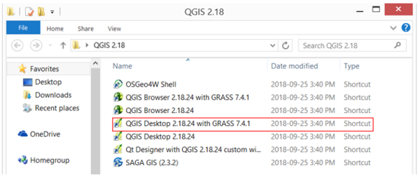
Once the installation of QGIS has completed, you’ll have to find the application either on your desktop or through your file explorer. In my case, going through the file explorer brings me to the following folder. (Figure 2)
Note, that by using the default settings in the download application, this folder was located here: "C:\Users\Public\Desktop\QGIS 2.18" on my computer. This may be the case for you as well, although it may be at a different root directory then C. You can also access this file by clicking the shortcut that the download should create on your dashboard. (Figure 3)
For this tutorial, we’ll be using the “QGIS Desktop 2.18.24 with GRASS 7.4.1” (Figure 2) Double click on the application and QGIS will launch.
QGIS – Overview
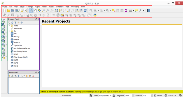
Once QGIS launches, you’ll be met with the user interface (UI). In order to get you somewhat acquainted with the interface before we start delving into TINs, DEMs and contours we’ll briefly describe the five main components that make up the UI. These components are highlighted in Figure 4 through the use of coloured blocks. All of the following colour coded sections refer to Figure 4.
Red: This area includes your toolbars and main menu (top left, twelve words). The main menu is the area used for most functions that don’t have an associated toolbar. For example, if in the subsequent tutorial instructions, you’re asked to go through the menu via the following path: “Layers /Create Layer / New Shapefile Layer” this would mean to go through the Layers main menu option and follow the subsequent selections. This is what the above path would look like in the QGIS GUI:
Toolbars comprise the icons below the main menu. These play a similar role to the main menu, except that each toolbar focuses on a specific task with related functions and uses icons instead of words. For example, the aptly named “Map Navigation Toolbar” gives users easy to understand navigation tools in one place. (Figure 6)
Green: This is the “Manage Layers Toolbar”. The purpose of this is to quickly add new layers in many different formats. For example, if you wanted to add a raster layer, you would simply click the “Add Raster Layer” button ![]() . This plays an important role in starting any type of spatial data display.
. This plays an important role in starting any type of spatial data display.
Purple: For the limited purposes of this tutorial, the “Browser Panel” is simply that, a way to access files on your computer within QGIS. You can easily access any type of file within this window.
Blue: The “Layer Panel” is an area where the user can view the layers they have open in QGIS. Any files you load into QGIS will appear here. You can turn on/off all layers, modify their display order and look at their properties in this panel. This is an essential and thankfully easy to use panel for any activities involving QGIS.
Yellow: This is simply the display panel. Any spatial information will appear here so long as the layer is turned on.
Elevation Display Datatypes
Now that we have a basic idea of what QGIS is, why it’s important and how to get it running we’ll start manipulating data to create our three types of elevation display data. It’s important to understand these three display types as they all use data types that are ubiquitous in GIS and are the most common way of displaying elevation in GIS.
TINs (Triangular Irregular Networks)
What are TINs?
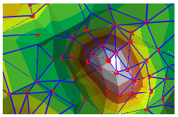
TINs are a way of displaying the elevation of a surface. They use vector point data which have x, y and z values associated with them. The x and y locate the 2 dimensional location of the point, while the z gives the elevation of the point. Z data is important because without it the TIN has no real meaning. The points supplied are connected to their neighbours by triangles giving the process its namesake. Using a TIN means that detail within the connecting triangles may be lost, however, they can represent elevation with relatively few points.
Data Import
In order to create a TIN, we need to import a point cloud that contains z values. The data we are going to use can be found here within the CUOSGwiki. Simply click the download and place the file into a folder named tutorial. The file should be called “Dot_Heights.shp”, right click on the folder and left click “Rename”. Name the folder “Carleton Elevation” and hit enter. Now, you’ll need to unzip the file. Left click on the folder, go to “Extract All” and right click. A tool will open entitled “Extract Compressed (Zipped) Folders”, leave all of the inputs as they are and click extract. Finally, delete the old zipped folder. In the end, your folder should look like this (Figure 8) and it should be located in a directory similar to this (C:\Users\YourUserName\Documents\Tutorial).
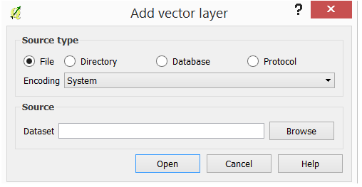
Now that the elevation file is on your computer, we can import it into QGIS. To do this, go to the “Manage Layers Toolbar” (Green) and click the “Add Vector Layer” icon ![]() . This will open the “Add Vector Layer” tool. (Figure 9)
. This will open the “Add Vector Layer” tool. (Figure 9)
Ensure that under “Source type” the inputs are set to “File” and “System” as shown above. Once this is complete left click on the browse button and navigate to the area of the “Carleton Elevation” folder were all the SHPs, SHXs and DBFs are stored. Once there, double click on the DBF. (Figure 10)
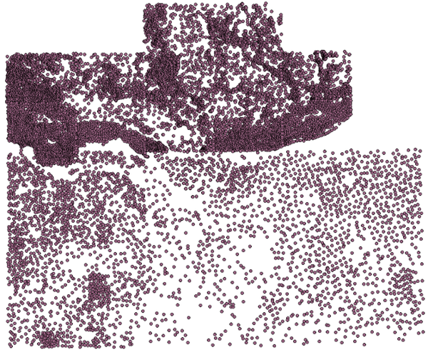
Once this is complete, simply click “Open” in the “Add Vector Layer” tool. The point elevation cloud should open in the “Display Panel” (Yellow) and the title of the layer should be in the “Layers Panel” (Blue). It should look something like this, though the colour may vary. (Figure 11)
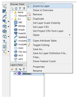
If there is no image displaying in the “Display Panel” go to the “Layers Panel” (Blue) and ensure that the layer is appearing there. If it is, right click on it and hit “Zoom to Layer”. This should bring you to the points if they are outside of our extent. (Figure 12)
If the layer is not there, simply repeat the previous steps in this section. Now that your data is imported into QGIS we can create a TIN.
Creating a TIN
QGIS is unable to create 3D TINs, this would require the use of GRASS which is beyond the scope of this tutorial. However, we can create a Delaunay Triangulation and a raster representation of elevation based on this Delaunay Triangulation instead. Delaunay Triangulation will connect nearest neighbor points to each other, however this will not represent elevation in 2 dimensions. This is why we have to rely on the derived raster layer when working in 2 dimensions.
Delaunay Triangulation
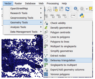
First, we will create our Delaunay Triangles in order to see how the process works. We will do this by going to the “Vector” selection in the main menu (red) and navigating to Vector/Geometry Tools/Delaunay Triangulation. (Figure 13)
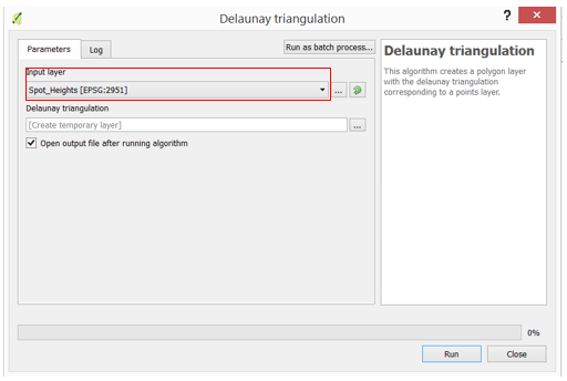
Once clicked, the “Delaunay Triangulation” tool will launch. Ensure that the layer we added earlier is selected in the input layer. (Figure 14)
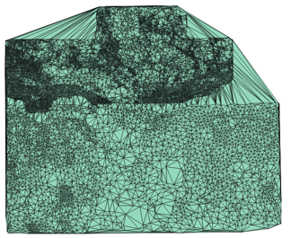
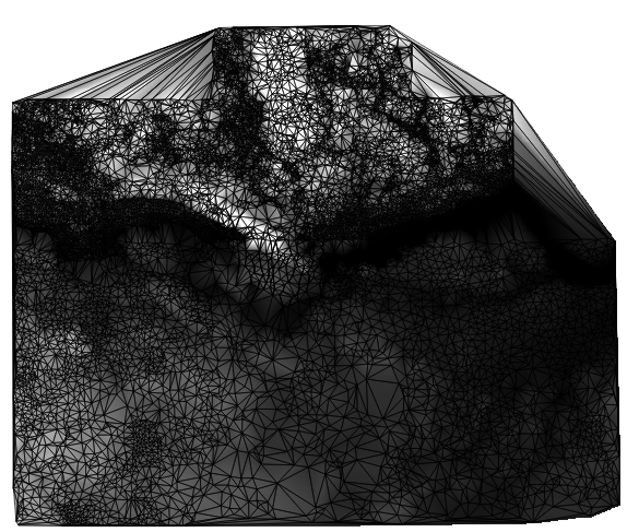
Once this is complete, simply click the “Run” button. The processing may take a few minutes and QGIS may become unresponsive. Avoid clicking in QGIS during processing. A second layer should appear on top of the “Spot_Heights” layer in the “Layers Panel” (Blue) and “Display Panel” (Yellow). Notice that the new layer named “Delaunay Triangulation” consists of triangles connecting our point to their neighboring points. (Figure 15)
In a 3D TIN there would be a change in angle of the lines connecting the points to represent elevation increase and decrease. Unfortunately, QGIS does not support this. As a result the TIN we produced does not tell us anything about elevation. Now we will create a raster representation of elevation, using a Delaunay Triangulation method, to represent the elevation.
DEMs (Digital Elevation Model)
What are DEMs?
A DEM is a digital representation of the earth’s surface. There are typically two types of DEMs, a DTM (Digital Terrain Model) and a DSM (Digital Surface Model). A DTM is a representation a ground surface that does not include vegetation or buildings, while a DSM includes everything captured in the elevation data. The data you’ve downloaded is a surface model that has had a vegetation removal algorithm run on it. This means we will be creating a DTM. A DEM uses elevation data to create a raster output. In order to add readable elevation to our triangles, we’re going to create a DTM.
Plugin
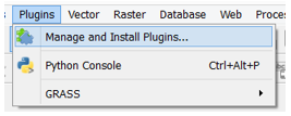
First, we have to activate the “Interpolation Plugin” to do the raster function we want. To do this, go to the “Plugins” selection on the main menu (Red) and click the “Manage and Install Plugins…” This will open the “Plugins” tool. (Figure 16)
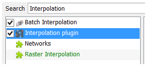
Within the tool, type “Interpolation” into the top search engine. This should narrow the list of plugins. Select the “Interpolation plugin” by checking the box to its left. Once this is done, click the “Close” button in the bottom right. (Figure 17)
DEM - Raster Creation
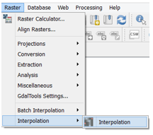
Now that the “Interpolation plugin” is installed, we need to launch it and set the proper parameters that will create a raster representation of the point cloud using Delaunay Triangulation. To open the plugin, simply go to the “Raster” option in the main menu (Red) and follow the path Raster/Interpolation/interpolation. This will open the “Interpolation plugin” tool. (Figure 18)
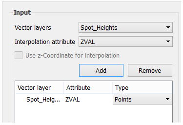
In the tool under “Inputs”, ensure that “Vector Layers” is set to “Spot_Height” because this is the layer with elevation points. Set “Interpolation attribute” to “ZVAL” because this is the column in our layer attributes that has the elevation data. Once this is done, click the add button. This should make the layer and attribute appear in the table below. (Figure 19)
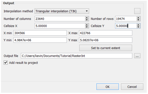
Under the “Output” section of the tool ensure that “Interpolation method” is set to “TIN” as having it set to another option will not use Delaunay Triangulation to make the raster. Maintain the size of the “Number of columns” and rows at “300”. The “Cellsize X” and Y determine the size of the pixels in the raster. Larger datasets may require larger cells to reduce system stress. We have a relatively small dataset, so let’s set our cell size to “200”. The extents of the interpolation are automatically set to those of the inputted dataset(s), meaning we can leave them at their default. It’s worth noting that if you only want to interpret a certain area, you can zoom to the desired extent and click “set to current extent”. Finally, place the “Output file” in the Tutorial folder under the name “RasterInt”.
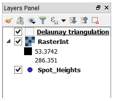
Once these inputs are complete, click “OK”. Once processing completes, a third layer will enter the “Layer Panel” and be displayed in the “Display Panel”. The low points will be displayed as black and the high as white on a grey scale. By looking at the “Layers Panel”, we can see that the lowest point is 53 m and the highest is 286 m. (Figure 21)
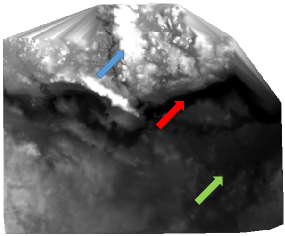
By looking at the layer, we can make out certain features. The data is of elevation points taken from Ottawa/Gatineau, Canada. We can see the lowlands of the city area, the lowest (black) area representing the river and the high (white) areas which are the hills of Gatineau. (Figure 22)
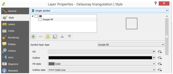
If we go into the “Layers Panel” and by clicking and dragging our “Delaunay triangulation” layer above our “RasterInt” layer we can see the impact of the Delaunay Triangulation. Double click on the “Delaunay triangulation” to open the attribute table. One the “Layer property” tool is open, navigate to the “Style” category. Double click on “Simple fill” in the upper left. This should open the “Symbol layer type” options. Under “Fill” set the type to transparent fill. (Figure 23)
Now in the “Display Panel” we can see the “RasterInt” layer under the “Delaunay triangulation” layer. You can see that the patterns of elevation in the “RasterInt” match closely to those in “Delaunay triangulation” because they both use the same process. (Figure 24)
This is the easiest and most useful way of creating a 2D TIN within QGIS. The raster used to represent elevation makes the output a raster instead of vector as a pure 3D TIN would be.
Contours
What are Contours?
Contours are the traditional way of representing elevation in a paper map. The contour is a line that represents a continuous elevation. The proximity of a contour to its neighbours indicates steepness of slope. Two contours close together represents a steep slope, while contours far apart indicates a smooth slope. If an area has very few contours, it is likely a flat area. Creating contours is easy once we have a raster layer. Though contours are used less now than in the past and do not represent continuous elevation as well as DEMs or TINs, they still do a good job of getting elevation and slope across to an audience. They are simple to understand and can be easier for individuals whose last contact with mapping techniques was in high school. Many maps are still being digitized from physical maps with contours, so understanding them in QGIS is important.
Creating Contours
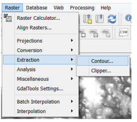
First, make sure that “RasterInt” is still in the “Layers Panel” (Blue) because we need a raster layer to create the contours. Go to “Raster” in the main menu (Red) and follow the path Raster/Extraction/Contour. (Figure 25)
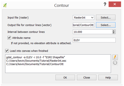
This will open the “Contour” tool. Ensure that “Input file (raster)” is set to the raster layer “RasterInt”. Set the “Output value” to the “Tutorial” folder and name it “ContourOtt”. The “Interval between contour lines” determines how far the distance between each contour will be. This is up to you, but bear in mind that too many contours can clutter a map and two few can make discerning slope difficult. The default of “10” is usually a good starting point. Check the “Attribute name” box and set it to “Elev”. This will tell the tool where to source the elevation information. Finally, hit the “OK” button. (Figure 26)
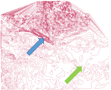
A layer named “ContourOtt contour Line” will be created. We can see that the lines are closest together in the hills near Gatineau and farthest apart in the lowlands near Ottawa. (Figure 27)
Conclusion
By completing this tutorial, you’ve learned many of the basic aspects required to use QGIS, including how to activate plugins, all of the main panels and general GUI navigation. You’ve also learned about TINs, DEMs and contours, which comprise the main ways of representing elevation in 2D and how to create them in QGIS using point clouds.
