Interferometry in ISCE with ALOS Imagery
The InSAR Scientific Computing Environment (ISCE) was developed by NASA for the purpose of processing Interferometric Synthetic Aperture Radar imagery from a variety of earth observation satellites. The open source software was designed from the ground up and is primarily based in the Python programming language. The software can be used to create an interferogram, a type of raster image that measures the phase change between two separate image acquisitions of the same region on earth. From the phase changes, information about surface deformations can be interpreted.
One of the many applications of interferometry is the study of volcanic activity. The example used in this tutorial is the March 2011 Kilauea Volcano.
ISCE does not offer a Graphical User Interface(GUI) and so, although it is not necessary, some experience with the following tasks is recommended:
- Using the Command Line (Terminal);
- Setting up a Conda environment;
- Writing and executing scripts in Python.
Note: this tutorial is only compatible with Linux and MacOS. ISCE is not currently supported on a Windows environment.
Contents
Download the Data
Estimated Time: 30min-1hr depending on your internet connection's download speed
EarthData Account Setup
ALOS is the "Advanced Land Observation Satellite" developed by JAXA. It has three remote sensing instruments on board, one of which is the Phased Array type L-band Synthetic Aperture Radar (PALSAR). Imagery from this sensor can be obtained freely from the Alaska Satellite Facility (ASF) with an Earth Data account.
Please follow the link below to register for an Earth Data account now, or verify that you are registered:
Once you have verified your account, you will be able to automatically download the data by running the script at the end of this section. To run some of the functions in ISCE and to download the data with the provided script, you will need a file on your computer that stores your Earth Data Account credentials. To do this, run the following commands, replacing YOURUSERNAME and YOURPASSWORD with your Earth Data login information:
 cd ~
 touch .netrc
 echo "machine urs.earthdata.nasa.gov login YOURUSERNAME password YOURPASSWORD " > .netrc
 chmod 0600 .netrc
This creates a .netrc file that stores your user credentials with special permissions so that they may only be accessed by certain methods. To learn more about this step, follow this link.
Automated Download
Copy and paste the following script into your favorite python IDE (or any text editor) and save it as setup.py in your preferred directory. This script will set up a working directory to store all the processed files in and will also download the required data from ASF. It will take some time for the data to download, so feel free to move on to the Installation section while you are waiting.
# This script downloads the data from the Alaska Satellite Facility webpage that
# be used in the "Interferometry in ISCE with ALOS Imagery" tutorial
# author@allyplourde created on 12-08-2020 10:40:00

import os

# setup the working directory:
home_dir = os.path.join(os.getenv("HOME"), "GEOM4008_ISCE_Tutorial")
PROCESS_DIR = os.path.join(home_dir, "Hawaii_ALOS1")
DATA_DIR =  os.path.join(PROCESS_DIR, "data")

# read EarthData credentials from ~/.netrc file
if (os.path.exists(os.path.join(os.getenv("HOME"), ".netrc"))):
    netrc_path = os.path.join(os.getenv("HOME"), ".netrc")
    count = len(open(netrc_path).readlines(  ))
    if count == 1:
        file = open(os.path.join(os.getenv("HOME"), ".netrc"), "r")
        contents = file.read().split(" ")
        ASF_USER = contents[3]
        ASF_PASS = contents[5]
        file.close()
    else:
        ASF_USER = np.loadtxt(os.path.join(os.getenv("HOME"), ".netrc"), skiprows=1, usecols=1, dtype=str)[0]
        ASF_PASS = np.loadtxt(os.path.join(os.getenv("HOME"), ".netrc"), skiprows=1, usecols=1, dtype=str)[1]
else:
    print("WARNING: The ASF USER pass needs to be included in ~/.netrc file.")
    print(" The ~/.netrc file does not exist or is not setup properly.")

# set up internal directories to keep data organized
if not os.path.exists(PROCESS_DIR):
    print("create ", PROCESS_DIR)
    os.makedirs(PROCESS_DIR)
else:
    print(PROCESS_DIR, " already exists!")

if not os.path.exists(DATA_DIR):
    print("create ", DATA_DIR)
    os.makedirs(DATA_DIR)
else:
    print(DATA_DIR, " already exists!")

# change working directory to data directory to
# prepare for file downloads
os.chdir(DATA_DIR)

cmd = "wget  https://datapool.asf.alaska.edu/L1.0/A3/ALPSRP265743230-L1.0.zip --user={0} --password={1}".format(ASF_USER, ASF_PASS)
if not os.path.exists(os.path.join(DATA_DIR, "ALPSRP265743230-L1.0.zip")):
    os.system(cmd)
else:
    print("ALPSRP265743230-L1.0.zip already exists")

cmd = "wget  https://datapool.asf.alaska.edu/L1.0/A3/ALPSRP272453230-L1.0.zip --user={0} --password={1}".format(ASF_USER, ASF_PASS)
if not os.path.exists(os.path.join(DATA_DIR, "ALPSRP272453230-L1.0.zip")):
   os.system(cmd)
else:
   print("ALPSRP272453230-L1.0.zip already exists")
Installation
Estimated Time: ~30 min to install Anaconda; ~30 min to install ISCE Environment'
A Conda environment will be used to manage software dependencies. In order to use the Conda environment Anaconda needs to be installed, click here for instructions on installing Anaconda. Once Anaconda is installed, open a new terminal and enter the command:
conda init
this sets up a base Anaconda environment that will allow you to access certain commands and libraries directly from the command line.
ISCE2 Environment Setup
ISCE-2 has a number of dependencies and is highly susceptible to versioning conflicts. By using a virtual environment, the packages (and their versions) will be uploaded to a separate space on your computer rather than in the root file. An environment configured for ISCE-2 has been uploaded to the Anaconda cloud, to create this environment locally, execute the following command:
conda env create allyplourde/ISCE2
Shortly after running the command, you should see packages beginning to be installed one by one.
This step may take a while to complete. While waiting, you can click here to learn more about this step. The Conda environment is stored in a YAML file on the cloud. These files can be created in any text editor by saving them with the .yml extension. The computer interprets the file to determine what to name the environment, where to download packages from, and what packages need to be installed. The contents of the ISCE2 environment being downloaded from the cloud are shown below.
| name: ISCE2
channels: - conda-forge - defaults dependencies: - python=3.6 - isce2 - git - tqdm |
Activation and Testing
Once the installation is complete, the environment must be activated using the following command
conda activate ISCE-2
you can observe that the <ISCE-2> environment is now pre-pended to the working directory path.
Creating the ISCE-2 Conda environment has already taken care of its installation as well as setting some global variables. To confirm ISCE-2 has been successfully installed, use this echo command:
echo $ISCE_HOME
This should output the path to the folder where ISCE-2 has been installed
Finally, to test the installation, run the following command:
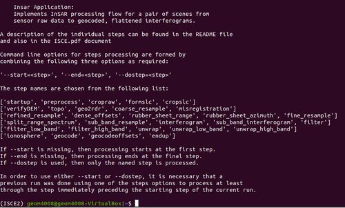
python $ISCE_HOME/applications/stripmapApp.py --help --steps
This will output information about the stripmapApp python application including a description and configuration guidelines. This is the application that will be used to create an interferogram with our two images. Take a minute to review the output.
Processing
Estimated Time: ~1-2 hr
Configuration
ISCE-2 uses XML a set of XML files to configure the processing steps. The setup of the configuration files has been automated for this tutorial for the data downloaded previously. For more information on setting up configuration files, refer to reference files provided on the isce-2 GitHub repository: https://github.com/isce-framework/isce2/tree/main/examples/input_files. The automated script is provided below.
import os

def configure_inputs(outDir):

    """Write Configuration files for ISCE2 stripmapApp to process NISAR sample products"""
    cmd_reference_config = '<component>\n \
    <property name="IMAGEFILE">\n \
       <value>[data/20110119/ALPSRP265743230-L1.0/IMG-HH-ALPSRP265743230-H1.0__D]</value>\n\
    </property>\n\
    <property name="LEADERFILE">\n\
        <value>[data/20110119/ALPSRP265743230-L1.0/LED-ALPSRP265743230-H1.0__D]</value>\n\
    </property>\n\
    <property name="OUTPUT">\n\
        <value>20110119</value>\n\
    </property>\n\
    </component>'

    print("writing reference.xml")
    with open(os.path.join(outDir,"reference.xml"), "w") as fid:
        fid.write(cmd_reference_config)

    cmd_secondary_config = '<component>\n \
    <property name="IMAGEFILE">\n \
        <value>[data/20110306/ALPSRP272453230-L1.0/IMG-HH-ALPSRP272453230-H1.0__D]</value>\n \
    </property>\n \
    <property name="LEADERFILE">\n \
        <value>[data/20110306/ALPSRP272453230-L1.0/LED-ALPSRP272453230-H1.0__D]</value>\n \
    </property>\n \
    <property name="OUTPUT">\n \
        <value>20110306</value>\n \
    </property>\n \
    </component>\n '

    print("writing secondary.xml")
    with open(os.path.join(outDir,"secondary.xml"), "w") as fid:
        fid.write(cmd_secondary_config)

    try:

        cmd_stripmap_config = '<?xml version="1.0" encoding="UTF-8"?>\n \
		<stripmapApp>\n \
		  <component name="insar">\n \
		    <property name="sensor name">ALOS</property>\n \
		    <component name="reference">\n \
			<catalog>reference.xml</catalog>\n \
		    </component>\n \
		    <component name="secondary">\n \
			<catalog>secondary.xml</catalog>\n \
		    </component>\n \
		\n \
		    <!--\n \
		    <property name="demFilename">\n \
			<value>demLat_N18_N21_Lon_W156_W154.dem.wgs84</value>\n \
		    </property>\n \
		    -->\n \
		\n \
		    <property name="unwrapper name">icu</property>\n \
		\n \
		    <property name="do split spectrum">False</property>\n \
		\n \
		    <property name="do dispersive">False</property>\n \
		\n \
		</component>\n \
		</stripmapApp>'

        print("writing stripmapApp.xml")
        with open(os.path.join(outDir,"stripmapApp.xml"), "w") as fid:
            fid.write(cmd_stripmap_config)
    except:
        print("OH no! something has gone wrong!")

if __name__ == "__main__":
	# setup the working directory:
	home_dir = os.path.join(os.getenv("HOME"), "Tutorial")
	PROCESS_DIR = os.path.join(home_dir, "Hawaii_ALOS1")
	DATA_DIR =  os.path.join(PROCESS_DIR, "data")


	os.chdir(PROCESS_DIR)

	configure_inputs(PROCESS_DIR)
Creating an Interferogram
ISCE-2 can be run from the command line. The following command already shown in the previous section provides some key information on how to interact with the software from the command line.
python $ISCE_HOME/applications/stripmapApp.py --help --steps
Near the bottom, the output provides information about the steps that need to be run to create an interferogram. It is important to follow these steps in the order they are listed in. The configuration file must specify certain variables for some steps to be used, otherwise they are skipped over; however, this is out of the scope of this tutorial, for more information, refer to the ISCE-2 GitHub repository.
These steps can be run one at a time using the following command
python $ISCE_HOME/applications/stripmapApp.py stripmapApp.xml --start=<STEP> --end=<STEP>
Recall, the $ISCE_HOME is the path variable pointing to where ISCE-2 has been installed, stripmapApp.py is the Python application that will be used to create the interferogram, and stripmapApp.xml is the XML file created in the configuration step. Multiple steps can also be run by simply setting the start and end variables accordingly. To run the complete processing flow, you can use the following command; however, keep in mind that this may take a few hours to complete. You may also want to ensure you have enough space on your machine to store all the files, it is recommended to have at least 25 GB free.
python $ISCE_HOME/applications/stripmapApp.py stripmapApp.xml --start=startup --end=endup
Output
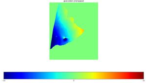
Now that the interferogram has been created, we need a way to display it. The images created in the above steps are stored VRT files, a type of virtual file used to save space. GDAL can be used to translate such files into a more familiar type such as a GeoTIFF. GDAL was automatically installed to the ISCE2 conda environment during the Installation step and can be imported as a python library. The image can also be quickly displayed using the Python library Matplotlib. A script to convert the interferogram to a .tif file as well as display it in Matplotlib has been provided below.
import gdal
import matplotlib.pyplot as plt

# reading the multi-looked wrapped interferogram
ds = gdal.Open("interferogram/filt_topophase.unw.geo", gdal.GA_ReadOnly)

ds = gdal.Translate('output.tif', ds)

unw_geocoded = ds.GetRasterBand(2).ReadAsArray()
ds = None


fig = plt.figure(figsize=(14,12))

ax = fig.add_subplot(1,1,1)
cax = ax.imshow(unw_geocoded, vmin = -15 , vmax = 15.0, cmap = 'jet')
ax.set_title("geocoded unwrapped")
ax.set_axis_off()
cbar = fig.colorbar(cax, ticks=[-15,0, 15], orientation='horizontal')

plt.show()

unw_geocoded = None
Further Reading
For a detailed explanation on the process of creating Interferograms, try out this tutorial:
"Creating_Interferogram_for_Mapping_Earthquake_Deformation_by_using_Sentinel-1_Data_in_SNAP"
Visit the ISCE-2 GitHub Repository for additionally resources and examples:
https://github.com/isce-framework/isce2


